ovito.data
This Python module defines various data object types, which are produced and processed within OVITO’s data pipeline system.
It also provides the DataCollection class as a container for such data objects as well as several utility classes for
computing neighbor lists and iterating over the bonds connected to a particle.
Data containers:
DataObject- base of all data object types in OVITO
DataCollection- a general container for data objects representing an entire dataset
PropertyContainer- manages a set of uniformPropertyarrays
Particles- a specializedPropertyContainerfor particles
Bonds- specializedPropertyContainerfor bonds
VoxelGrid- specializedPropertyContainerfor 2d and 3d volumetric grids
DataTable- specializedPropertyContainerfor tabulated data
Lines- set of 3d line segments
Vectors- set of vector glyphs
Data objects:
Property- uniform array of property values
SimulationCell- simulation box geometry and boundary conditions
SurfaceMesh- polyhedral mesh representing the boundaries of spatial regions
TriangleMesh- general mesh structure made of vertices and triangular faces
DislocationNetwork- set of discrete dislocation lines with Burgers vector information
Auxiliary data objects:
ElementType- base class for type descriptors used in typed properties
ParticleType- describes a single particle or atom type
BondType- describes a single bond type
Utility classes:
CutoffNeighborFinder- finds neighboring particles within a cutoff distance
NearestNeighborFinder- finds N nearest neighbor particles
BondsEnumerator- lets you efficiently iterate over the bonds connected to a particle
- class ovito.data.BondType
Base:
ovito.data.ElementTypeRepresents a bond type. This class inherits all its fields from the
ElementTypebase class.You can enumerate the list of defined bond types by accessing the
bond_typesbond property object:bond_type_property = data.particles.bonds.bond_types for t in bond_type_property.types: print(t.id, t.name, t.color, t.radius)
- property radius: float
This attribute controls the display radius of all bonds of this type.
When set to zero, bonds of this type will be rendered using the standard width specified by the
BondsVis.radiusparameter. Furthermore, precedence is given to any per-bond widths assigned to theWidthbond property if that property exists.- Default:
0.0
Added in version 3.10.0.
- class ovito.data.Bonds
Base:
ovito.data.PropertyContainerStores the list of bonds and their properties. A
Bondsobject is always part of a parentParticlesobject. You can access it as follows:data = pipeline.compute() print("Number of bonds:", data.particles.bonds.count)
The
Bondsclass inherits thecountattribute from itsPropertyContainerbase class. This attribute returns the number of bonds.Bond properties
Bonds can be associated with arbitrary bond properties, which are managed in the
Bondscontainer as a set ofPropertydata arrays. Each bond property has a unique name by which it can be looked up:print("Bond property names:") print(data.particles.bonds.keys()) if 'Length' in data.particles.bonds: length_prop = data.particles.bonds['Length'] assert(len(length_prop) == data.particles.bonds.count)
New bond properties can be added using the
PropertyContainer.create_property()method.Bond topology
The
Topologybond property, which is always present, defines the connectivity between particles in the form of a N x 2 array of indices into theParticlesarray. In other words, each bond is defined by a pair of particle indices.for a,b in data.particles.bonds.topology: print("Bond from particle %i to particle %i" % (a,b))
Note that the bonds of a system are not stored in any particular order. If you need to enumerate all bonds connected to a certain particle, you can use the
BondsEnumeratorutility class for that.Bonds visualization
The
Bondsdata object has aBondsViselement attached to it, which controls the visual appearance of the bonds in rendered images. It can be accessed through thevisattribute:data.particles.bonds.vis.enabled = True data.particles.bonds.vis.flat_shading = True data.particles.bonds.vis.width = 0.3
Computing bond vectors
Since each bond is defined by two indices into the particles array, we can use these indices to determine the corresponding spatial bond vectors connecting the particles. They can be computed from the positions of the particles:
topology = data.particles.bonds.topology
positions = data.particles.positions
bond_vectors = positions[topology[:,1]] - positions[topology[:,0]]
Here, the first and the second column of the bonds topology array are used to index into the particle positions array. The subtraction of the two indexed arrays yields the list of bond vectors. Each vector in this list points from the first particle to the second particle of the corresponding bond.
Finally, we may have to correct for the effect of periodic boundary conditions when a bond connects two particles on opposite sides of the box. OVITO keeps track of such cases by means of the special
Periodic Imagebond property. It stores a shift vector for each bond, specifying the directions in which the bond crosses periodic boundaries. We make use of this information to correct the bond vectors computed above. This is done by adding the product of the cell matrix and the shift vectors from thePeriodic Imagebond property:bond_vectors += numpy.dot(data.cell[:3,:3], data.particles.bonds.pbc_vectors.T).T
The shift vectors array is transposed here to facilitate the transformation of the entire array of vectors with a single 3x3 cell matrix. To summarize: In the two code snippets above, we have performed the following calculation of the unwrapped vector \(\mathbf{v}\) for every bond (a, b) in parallel:
\(\mathbf{v} = \mathbf{x}_b - \mathbf{x}_a + \mathbf{H} \cdot (n_x, n_y, n_z)^{T}\),
with \(\mathbf{H}\) denoting the simulation cell matrix and \((n_x, n_y, n_z)\) the bond’s PBC shift vector.
Standard bond properties
The following standard properties are defined for bonds:
Property name
Python access
Data type
Component names
Bond Type
int32
Color
float32
R, G, B
Length
float64
Particle Identifiers
int64
A, B
Periodic Image
int32
X, Y, Z
Selection
int8
Topology
int64
1, 2
Transparency
float32
Width
float32
- add_bond(a, b, type=None, pbcvec=None)
Creates a new bond between two particles a and b, both parameters being indices into the particles list.
- Parameters:
a (int) – Index of first particle connected by the new bond. Particle indices start at 0.
b (int) – Index of second particle connected by the new bond.
type (int | None) – Optional type ID to be assigned to the new bond. This value will be stored to the
bond_typesarray.pbcvec (tuple[int, int, int] | None) – Three integers specifying the bond’s crossings of periodic cell boundaries. The information will be stored in the
pbc_vectorsarray.
- Returns:
The 0-based index of the newly created bond, which is
(Bonds.count-1).- Return type:
The method does not check if there already is an existing bond connecting the same pair of particles.
The method does not check if the particle indices a and b do exist. Thus, it is your responsibility to ensure that both indices are in the range 0 to
(Particles.count-1).In case the
SimulationCellhas periodic boundary conditions enabled, and the two particles connected by the bond are located in different periodic images, make sure you provide the pbcvec argument. It is required so that OVITO does not draw the bond as a direct line from particle a to particle b but as a line passing through the periodic cell faces. You can use theParticles.delta_vector()function to compute pbcvec or use thepbc_shiftvector returned by theCutoffNeighborFinderutility.
- property bond_types: Property | None
The
Propertydata array for theBond Typestandard bond property; orNoneif that property is undefined.
- property colors: Property | None
The
Propertydata array for theColorstandard bond property; orNoneif that property is undefined.
- property pbc_vectors: Property | None
The
Propertydata array for thePeriodic Imagestandard bond property; orNoneif that property is undefined.
- property selection: Property | None
The
Propertydata array for theSelectionstandard bond property; orNoneif that property is undefined.
- property topology: Property | None
The
Propertydata array for theTopologystandard bond property; orNoneif that property is undefined.
- class ovito.data.BondsEnumerator(bonds: Bonds)
Utility class that permits efficient iteration over the bonds connected to specific particles.
The constructor takes a
Bondsobject as input. From the generally unordered list of bonds, theBondsEnumeratorwill build a lookup table for quick enumeration of bonds of particular particles.All bonds connected to a specific particle can be subsequently visited using the
bonds_of_particle()method.Warning: Do not modify the underlying
Bondsobject while theBondsEnumeratoris in use. Adding or deleting bonds would render the internal lookup table of theBondsEnumeratorinvalid.Usage example
from ovito.io import import_file
from ovito.data import BondsEnumerator
from ovito.modifiers import ComputePropertyModifier

# Load a dataset containing atoms and bonds.
pipeline = import_file('input/bonds.data.gz', atom_style='bond')

# For demonstration purposes, let's define a compute modifier that calculates the length
# of each bond, storing the results in a new bond property named 'Length'.
pipeline.modifiers.append(ComputePropertyModifier(operate_on='bonds', output_property='Length', expressions=['BondLength']))

# Obtain pipeline results.
data = pipeline.compute()
positions = data.particles.positions  # array with atomic positions
bond_topology = data.particles.bonds.topology  # array with bond topology
bond_lengths = data.particles.bonds['Length']     # array with bond lengths

# Create bonds enumerator object.
bonds_enum = BondsEnumerator(data.particles.bonds)

# Loop over atoms.
for particle_index in range(data.particles.count):
    # Loop over bonds of current atom.
    for bond_index in bonds_enum.bonds_of_particle(particle_index):
        # Obtain the indices of the two particles connected by the bond:
        a = bond_topology[bond_index, 0]
        b = bond_topology[bond_index, 1]

        # Bond directions can be arbitrary (a->b or b->a):
        assert(a == particle_index or b == particle_index)

        # Obtain the length of the bond from the 'Length' bond property:
        length = bond_lengths[bond_index]

        print("Bond from atom %i to atom %i has length %f" % (a, b, length))
- class ovito.data.CutoffNeighborFinder(cutoff, data_collection)
A utility class that computes particle neighbor lists.
This class lets you iterate over all neighbors of a particle that are located within a specified spherical cutoff. You can use it to build neighbor lists or perform computations that require neighbor vector information.
The constructor takes a positive cutoff radius and a
DataCollectionproviding the input particles and theSimulationCell(needed for periodic systems).Once the
CutoffNeighborFinderhas been constructed, you can call itsfind()method to iterate over the neighbors of a particle, for example:from ovito.io import import_file from ovito.data import CutoffNeighborFinder # Load input simulation file. pipeline = import_file("input/simulation.dump") data = pipeline.compute() # Initialize neighbor finder object: cutoff = 3.5 finder = CutoffNeighborFinder(cutoff, data) # Prefetch the property array containing the particle type information: ptypes = data.particles.particle_types # Loop over all particles: for index in range(data.particles.count): print("Neighbors of particle %i:" % index) # Iterate over the neighbors of the current particle: for neigh in finder.find(index): print(neigh.index, neigh.distance, neigh.delta, neigh.pbc_shift) # The index can be used to access properties of the current neighbor, e.g. type_of_neighbor = ptypes[neigh.index]
Note: If you want to determine the N nearest neighbors of a particle, use the
NearestNeighborFinderclass instead.- Parameters:
cutoff (float)
data_collection (DataCollection)
- find(index)
Returns an iterator over all neighbors of the given particle.
- Parameters:
index (int) – The zero-based index of the central particle whose neighbors should be enumerated.
- Returns:
A Python iterator that visits all neighbors of the central particle within the cutoff distance. For each neighbor the iterator returns an object with the following property fields:
index: The zero-based global index of the current neighbor particle.
distance: The distance of the current neighbor from the central particle.
distance_squared: The squared neighbor distance.
delta: The three-dimensional vector connecting the central particle with the current neighbor (taking into account periodicity).
pbc_shift: The periodic shift vector, which specifies how often each periodic boundary of the simulation cell is crossed when going from the central particle to the current neighbor.
- Return type:
The index value returned by the iterator can be used to look up properties of the neighbor particle, as demonstrated in the example above.
Note that all periodic images of particles within the cutoff radius are visited. Thus, the same particle index may appear multiple times in the neighbor list of the central particle. In fact, the central particle may be among its own neighbors in a small periodic simulation cell. However, the computed vector (
delta) and PBC shift (pbc_shift) will be unique for each visited image of the neighbor particle.
- find_all(indices=None, sort_by=None)
This is a vectorized version of the
find()method, computing the neighbor lists and neighbor vectors of several particles in a single operation. Thus, this method can help you avoid a slow, nested Python loop in your code and it will make use of all available processor cores. You can request the neighbor lists for the whole system in one go, or just for a specific subset of particles given by indices.The method produces a uniform array of neighbor list entries. Each entry comprises a pair of indices, i.e. the central particle and one of its neighboring particles within the cutoff distance, and the corresponding spatial neighbor vector in 3d Cartesian coordinates. For best performance, the method returns all neighbors of all particles as one large array, which is unsorted by default (sort_by =
None). That means the neighbors of central particles will not form contiguous blocks in the output array; entries belonging to different central particles may rather appear in intermingled order!Set sort_by to
'index'to request grouping the entries in the output array based on the central particle index. That means each particle’s neighbor list will be output as a contiguous block. All blocks are stored back-to-back in the output array in ascending order of the central particle index or, if parameter indices was specified, in that order. The ordering of neighbor entries within each block will still be arbitrary though. To change this, set sort_by to'distance', which additionally sorts the neighbors of each particle by increasing distance.The method returns two NumPy arrays:
neigh_idx: Array of shape (M, 2) containing pairs of indices of neighboring particles, with M equal to the total number of neighbors in the system. Note that the array will contain symmetric entries (a, b) and (b, a) if neighbor list computation was requested for both particles a and b and they are within reach of each other.neigh_vec: Array of shape (M, 3) containing the xyz components of the Cartesian neighbor vectors (“delta”), which connect the M particle pairs stored inneigh_idx.- Parameters:
indices (Optional[ArrayLike]) – List of zero-based indices of central particles for which the neighbor lists should be computed. If left unspecified, neighbor lists will be computed for every particle in the system.
sort_by (Optional[Literal['index', 'distance']]) – One of “index” or “distance”. Requests ordering of the output arrays based on central particle index and, optionally, neighbor distance. If left unspecified, neighbor list entries will be returned in arbitrary order.
- Returns:
(neigh_idx, neigh_vec)- Return type:
Tip
Sorting of neighbor lists will incur an additional runtime cost and should only be requested if necessary. In any case, however, this vectorized method will be much faster than an equivalent Python for-loop invoking the
find()method for each individual particle.Attention
The same index pair (a, b) may appear multiple times in the list
neigh_idxif theSimulationCelluses periodic boundary conditions and its size is smaller than twice the neighbor cutoff radius. Note that, in such a case, the corresponding neighbor vectors inneigh_vecwill still be unique, because they are computed for each periodic image of the neighbor b.Added in version 3.8.1.
- find_at(coords)
Returns an iterator over all particles located within the spherical range of the given center position. In contrast to
find()this method can search for neighbors around arbitrary spatial locations, which don’t have to coincide with any physical particle position.- Parameters:
coords (ArrayLike) – A (x,y,z) coordinate triplet specifying the center location around which to search for particles.
- Returns:
A Python iterator enumerating all particles within the cutoff distance. For each neighbor the iterator returns an object with the following properties:
index: The zero-based global index of the current neighbor particle.
distance: The distance of the current particle from the center position.
distance_squared: The squared distance.
delta: The three-dimensional vector from the center to the current neighbor (taking into account periodicity).
pbc_shift: The periodic shift vector, which specifies how often each periodic boundary of the simulation cell is crossed when going from the center point to the current neighbor.
- Return type:
The index value returned by the iterator can be used to look up properties of the neighbor particle, as demonstrated in the example above.
Note that all periodic images of particles within the cutoff radius are visited. Thus, the same particle index may appear multiple times in the neighbor list. However, the computed vector (
delta) and image offset (pbc_shift) will be unique for each visited image of a neighbor particle.
- neighbor_distances(index: int) NDArray[float64]
Returns the list of distances between some central particle and all its neighbors within the cutoff range.
- Parameters:
index – The 0-based index of the central particle whose neighbors should be enumerated.
- Returns:
NumPy array containing the radial distances to all neighbor particles within the cutoff range (in arbitrary order).
This method is equivalent to the following code, but performance is typically a lot better:
def neighbor_distances(index):
    distances = []
    for neigh in finder.find(index):
        distances.append(neigh.distance)
    return numpy.asarray(distances)
- neighbor_vectors(index: int) NDArray[float64]
Returns the list of vectors from some central particle to all its neighbors within the cutoff range.
- Parameters:
index – The 0-based index of the central particle whose neighbors should be enumerated.
- Returns:
Two-dimensional NumPy array containing the vectors to all neighbor particles within the cutoff range (in arbitrary order).
The method is equivalent to the following code, but performance is typically a lot better:
def neighbor_vectors(index):
    vecs = []
    for neigh in finder.find(index):
        vecs.append(neigh.delta)
    return numpy.asarray(vecs)
- class ovito.data.DataCollection
Base:
ovito.data.DataObjectA
DataCollectionis a container class that holds together individual data objects, each representing different fragments of a dataset. For example, a dataset loaded from a simulation data file may consist of particles, simulation cell information, and additional auxiliary data such as the current time step number of the snapshots, etc. All this information is contained in oneDataCollection, which exposes the individual pieces of information as sub-objects, for example, via theDataCollection.particles,DataCollection.cell, andDataCollection.attributesfields.Data collections are the elementary entities that get processed within a data
Pipeline. Each modifier receives a data collection from the preceding modifier, alters it in some way, and passes it on to the next modifier. The output data collection of the last modifier in the pipeline is returned by thePipeline.compute()method.A data collection essentially consists of a bunch of
DataObjects, which are all stored in theDataCollection.objectslist. Typically, you don’t access the data objects list directly but rather use one of the special accessor fields provided by theDataCollectionclass, which give more convenient access to data objects of a particular kind. For example, theDataCollection.surfacesdictionary provides key-based access to all theSurfaceMeshinstances currently in the data collection.- apply(modifier, frame=None)
This method applies a
Modifierfunction to the data stored in this collection to modify it in place.- Parameters:
The method allows modifying a data collection with one of OVITO’s modifiers directly without the need to build up a complete
Pipelinefirst. In contrast to a data pipeline, theapply()method executes the modifier function immediately and alters the data in place. In other words, the original data in thisDataCollectiongets replaced by the output produced by the invoked modifier function. It is possible to first create a copy of the original data using theclone()method if needed. The following code example demonstrates how to useapply()to successively modify a dataset:from ovito.io import import_file from ovito.modifiers import * data = import_file("input/simulation.dump").compute() data.apply(RadialDistributionFunctionModifier(cutoff=2.9)) data.apply(ExpressionSelectionModifier(expression="Coordination<9")) data.apply(DeleteSelectedModifier())
Note that it is typically possible to achieve the same result by first populating a
Pipelinewith the modifiers and then calling itscompute()method at the very end:pipeline = import_file("input/simulation.dump") pipeline.modifiers.append(RadialDistributionFunctionModifier(cutoff=2.9)) pipeline.modifiers.append(ExpressionSelectionModifier(expression="Coordination<9")) pipeline.modifiers.append(DeleteSelectedModifier()) data = pipeline.compute()
An important use case of the
apply()method is in the implementation of a user-defined modifier function, making it possible to invoke other modifiers as sub-routines:# A user-defined modifier function that calls the built-in ColorCodingModifier # as a sub-routine to assign a color to each atom based on some property # created within the function itself: def modify(frame: int, data: DataCollection): data.particles_.create_property('idx', data=numpy.arange(data.particles.count)) data.apply(ColorCodingModifier(property='idx'), frame) # Set up a data pipeline that uses the user-defined modifier function: pipeline = import_file("input/simulation.dump") pipeline.modifiers.append(modify) data = pipeline.compute()
- property attributes: MutableMapping[str, Any]
This field contains a dictionary view with all the global attributes currently associated with this data collection. Global attributes are key-value pairs that represent small tokens of information, typically simple value types such as
int,floatorstr. Every attribute has a unique identifier such as'Timestep'or'ConstructSurfaceMesh.surface_area'. This identifier serves as lookup key in theattributesdictionary. Identifiers starting with'.'are hidden in the GUI. Attributes are dynamically generated by modifiers in a data pipeline or come from the data source. For example, if the input simulation file contains timestep information, the timestep number is made available by theFileSourceas the'Timestep'attribute. It can be retrieved from pipeline’s output data collection:>>> pipeline = import_file('snapshot_140000.dump') >>> pipeline.compute().attributes['Timestep'] 140000
Some modifiers report their calculation results by adding new attributes to the data collection. See each modifier’s reference documentation for the list of attributes it generates. For example, the number of clusters identified by the
ClusterAnalysisModifieris available in the pipeline output as an attribute namedClusterAnalysis.cluster_count:pipeline.modifiers.append(ClusterAnalysisModifier(cutoff = 3.1)) data = pipeline.compute() nclusters = data.attributes["ClusterAnalysis.cluster_count"]
The
ovito.io.export_file()function can be used to output dynamically computed attributes to a text file, possibly as functions of time:export_file(pipeline, "data.txt", "txt/attr", columns = ["Timestep", "ClusterAnalysis.cluster_count"], multiple_frames = True)
If you are writing your own modifier function, you let it add new attributes to a data collection. In the following example, the
CommonNeighborAnalysisModifierfirst inserted into the pipeline generates the'CommonNeighborAnalysis.counts.FCC'attribute to report the number of atoms that have an FCC-like coordination. To compute an atomic fraction from that, we need to divide the count by the total number of atoms in the system. To this end, we append a user-defined modifier function to the pipeline, which computes the fraction and outputs the value as a new attribute named'fcc_fraction'.pipeline.modifiers.append(CommonNeighborAnalysisModifier()) def compute_fcc_fraction(frame, data): n_fcc = data.attributes['CommonNeighborAnalysis.counts.FCC'] data.attributes['fcc_fraction'] = n_fcc / data.particles.count pipeline.modifiers.append(compute_fcc_fraction) print(pipeline.compute().attributes['fcc_fraction'])
- property cell: SimulationCell | None
Returns the
SimulationCelldata object describing the cell vectors and periodic boundary condition flags. It may beNone.Important
The
SimulationCelldata object returned by this attribute may be marked as read-only, which means your attempts to modify the cell object will raise a Python error. This is typically the case if the data collection was produced by a pipeline and its objects are owned by the system.If you intend to modify the
SimulationCelldata object within this data collection, use thecell_attribute instead to explicitly request a mutable version of the cell object. See topic Announcing object modification for more information. Usecellfor read access andcell_for write access, e.g.print(data.cell.volume) data.cell_.pbc = (True, True, False)
To create a
SimulationCellin a data collection that might not have a simulation cell yet, use thecreate_cell()method or simply assign a new instance of theSimulationCellclass to thecellattribute.
- clone()
Returns a shallow copy of this
DataCollectioncontaining the same data objects as the original.The method can be used to retain a copy of the original data before modifying a data collection in place, for example, using the
apply()method:original = data.clone() data.apply(ExpressionSelectionModifier(expression="Position.Z < 0")) data.apply(DeleteSelectedModifier()) print("Number of atoms before:", original.particles.count) print("Number of atoms after:", data.particles.count)
Note that the
clone()method performs an inexpensive shallow copy, meaning that the newly created collection still shares the data objects with the original collection.Keep in mind that data objects shared by two or more data collections are implicitly protected against modifications to avoid unexpected side effects. Thus, in order to subsequently modify the objects in either the original or the copy of the data collection, you have to use the underscore notation or the
DataObject.make_mutable()method to make a deep copy of the particular data object(s) you want to modify. For example:copy = data.clone() # Data objects are shared by original and copy: assert(copy.cell is data.cell) # In order to modify the SimulationCell in the dataset copy, we must request # a mutable version of the SimulationCell using the 'cell_' accessor: copy.cell_.pbc = (False, False, False) # As a result, the cell object in the second data collection has been replaced # with a deep copy and the two data collections no longer share the same # simulation cell object: assert(copy.cell is not data.cell)
Tip
The
clone()method is equivalent to the standard Python functioncopy.copy()when applied to aDataCollection. In fact, most OVITO object types can be shallow-copied with Python’scopy.copy()function and deep-copied with thecopy.deepcopy()function.- Return type:
- create_cell(matrix, pbc=(True, True, True), vis_params=None)
This convenience method conditionally creates a new
SimulationCellobject and stores it in this data collection. If a simulation cell already existed in the collection (cellis notNone), then that cell object is replaced with a modifiable copy if necessary and the matrix and PBC flags are set to the given values. The attachedSimulationCellViselement is maintained in this case.- Parameters:
matrix (ArrayLike) – A 3x4 array to initialize the cell matrix with. It specifies the three cell vectors and the origin.
pbc (tuple[bool, bool, bool]) – A tuple of three Booleans specifying the cell’s
pbcflags.vis_params (Mapping[str, Any] | None) – Optional dictionary to initialize attributes of the attached
SimulationCellViselement (only used if the cell object is newly created by the method).
- Return type:
The logic of this method is roughly equivalent to the following code:
def create_cell(data: DataCollection, matrix, pbc, vis_params=None) -> SimulationCell:
    if data.cell is None:
        data.cell = SimulationCell(pbc=pbc)
        data.cell[...] = matrix
        data.cell.vis.line_width = <...> # Some value that scales with the cell's size
        if vis_params:
            for name, value in vis_params.items(): setattr(data.cell.vis, name, value)
    else:
        data.cell_[...] = matrix
        data.cell_.pbc = pbc
    return data.cell_
Added in version 3.7.4.
- create_particles(*, vis_params=None, **params)
This convenience method conditionally creates a new
Particlescontainer object and stores it in this data collection. If the data collection already contains an existing particles object (particlesis notNone), then that particles object is replaced with a modifiable copy if necessary. The associatedParticlesViselement is preserved.- Parameters:
params (Any) – Key-value pairs passed to the method as keyword arguments are used to set attributes of the
Particlesobject (even if the particles object already existed).vis_params (Mapping[str, Any] | None) – Optional dictionary to initialize attributes of the attached
ParticlesViselement (only used if the particles object is newly created by the method).
- Return type:
The logic of this method is roughly equivalent to the following code:
def create_particles(data: DataCollection, vis_params=None, **params) -> Particles:
    if data.particles is None:
        data.particles = Particles()
        if vis_params:
            for name, value in vis_params.items(): setattr(data.particles.vis, name, value)
    for name, value in params.items(): setattr(data.particles_, name, value)
    return data.particles_
Usage example:
coords = [(-0.06,  1.83,  0.81), # xyz coordinates of the 3 particle system to create
          ( 1.79, -0.88, -0.11),
          (-1.73, -0.77, -0.61)]
particles = data.create_particles(count=len(coords), vis_params={'radius': 1.4})
particles.create_property('Position', data=coords)
Added in version 3.7.4.
- property dislocations: DislocationNetwork | None
Returns the
DislocationNetworkdata object; orNoneif there is no object of this type in the collection. Typically, theDislocationNetworkis created by a pipeline containing theDislocationAnalysisModifier.
- get(ref: Ref, require: bool = True, path: bool = False) DataObject | None
Resolves a
DataObject.Refreference by retrieving the referenced data object from thisDataCollection.- Parameters:
ref – The reference to the data object to be retrieved.
require – If
True, the method raises a KeyError if the referenced object does not exist in the data collection. IfFalse, the method returnsNonein the not-found case.path – If
True, the method returns a list of the data objects in the nested object hierarchy leading to the referenced object from the root of theDataCollection.
- Returns:
The referenced
DataObject, orNoneif require=False and the data object could not be found or if ref is a null reference.
An “underscore version” of this method is available, which should be used whenever you intend to modify the returned data object.
get_()implicitly callsmake_mutable()to ensure the data object can be modified without unexpected side effects.Added in version 3.11.0.
- property grids: Mapping[str, VoxelGrid]
Returns a dictionary view providing key-based access to all
VoxelGridsin this data collection. EachVoxelGridhas a uniqueidentifierkey, which allows you to look it up in this dictionary. To find out which voxel grids exist in the data collection and what their identifiers are, useprint(data.grids)
Then retrieve the desired
VoxelGridfrom the collection using its identifier key, e.g.charge_density_grid = data.grids['charge-density'] print(charge_density_grid.shape)
The view provides the convenience method
grids.create(), which inserts a newly createdVoxelGridinto the data collection. The method expects the uniqueidentifierof the new grid as first argument. All other keyword arguments are forwarded to the constructor to initialize the member fields of theVoxelGridclass:grid = data.grids.create( identifier="grid", title="Field", shape=(10,10,10), domain=data.cell)
If there is already an existing grid with the same
identifierin the collection, thecreate()method modifies and returns that existing grid instead of creating another one.
- property lines: Mapping[str, Lines]
A dictionary view providing key-based access to all
Linesobjects in this data collection. EachLinesobject has a uniqueidentifierkey, which can be used to look it up in the dictionary. You can useprint(data.lines)
to see which identifiers exist. Then retrieve the desired
Linesobject from the collection using its identifier key, e.g.lines = data.lines["trajectories"] print(lines["Position"])
The
Linesobject with the identifier"trajectories", for example, is the one that gets created by theGenerateTrajectoryLinesModifier.If you would like to create a new
Linesobject, in a user-defined modifier for instance, the dictionary view provides the methodlines.create(), which creates a newLinesand adds it to the data collection. The method expects the uniqueidentifierof the new lines object as first argument. All other keyword arguments are forwarded to the class constructor to initialize the member fields of theLinesobject:lines = data.lines.create(identifier="mylines")
If there is already an existing
Linesobject with the sameidentifierin the collection, thecreate()method returns that object instead of creating another one and makes sure it can be safely modified.
- property objects: MutableSequence[DataObject]
List of all top-level
DataObjectsin this data collection. You can add or remove data objects from this list as needed.Typically, however, you don’t need to work with this list directly, because the
DataCollectionclass provides several convenience accessor attributes for the different flavors of data objects in OVITO. For example,DataCollection.particlesreturns theParticlesobject (by looking it up in theobjectslist for you). Dictionary-like views such asDataCollection.tablesandDataCollection.surfacesprovide key-based access to particular kinds of data objects in the collection.To add new objects to the data collection, you can append them to the
objectslist or, more conveniently, use creation functions such ascreate_particles(),create_cell(), ortables.create(), which are provided by theDataCollectionclass.
- property particles: Particles | None
Returns the
Particlesobject, which manages all per-particle properties. It may beNoneif the data collection contains no particle model at all.Important
The
Particlesdata object returned by this attribute may be marked as read-only, which means attempts to modify its contents will raise a Python error. This is typically the case if the data collection was produced by a pipeline and all data objects are owned by the system.If you intend to modify the contents of the
Particlesobject in some way, use theparticles_attribute instead to explicitly request a mutable version of the particles object. See topic Announcing object modification for more information. Useparticlesfor read access andparticles_for write access, e.g.print(data.particles.positions[0]) data.particles_.positions_[0] += (0.0, 0.0, 2.0)
To create a new
Particlesobject in a data collection that might not have particles yet, use thecreate_particles()method or simply assign a new instance of theParticlesclass to theparticlesattribute.
- property surfaces: Mapping[str, SurfaceMesh]
Returns a dictionary view providing key-based access to all
SurfaceMeshobjects in this data collection. EachSurfaceMeshhas a uniqueidentifierkey, which can be used to look it up in the dictionary. See the documentation of the modifier producing the surface mesh to find out what the right key is, or useprint(data.surfaces)
to see which identifier keys exist. Then retrieve the desired
SurfaceMeshobject from the collection using its identifier key, e.g.surface = data.surfaces['surface'] print(surface.vertices['Position'])
The view provides the convenience method
surfaces.create(), which inserts a newly createdSurfaceMeshinto the data collection. The method expects the uniqueidentifierof the new surface mesh as first argument. All other keyword arguments are forwarded to the constructor to initialize the member fields of theSurfaceMeshclass:mesh = data.surfaces.create( identifier="surface", title="A surface mesh", domain=data.cell)
If there is already an existing mesh with the same
identifierin the collection, thecreate()method modifies and returns that existing mesh instead of creating another one.
- property tables: Mapping[str, DataTable]
A dictionary view of all
DataTableobjects in this data collection. EachDataTablehas a uniqueidentifierkey, which allows it to be looked up in this dictionary. Useprint(data.tables)
to find out which table identifiers are present in the data collection. Then use the identifier to retrieve the desired
DataTablefrom the dictionary, e.g.rdf = data.tables['coordination-rdf'] print(rdf.xy())
The view provides the convenience method
tables.create(), which inserts a newly createdDataTableinto the data collection. The method expects the uniqueidentifierof the new data table as first argument. All other keyword arguments are forwarded to the constructor to initialize the member fields of theDataTableclass:# Code example showing how to compute a histogram of the particles' x-coordinates within some interval. x_interval = (0.0, 100.0) x_coords = data.particles.positions[:,0] histogram = numpy.histogram(x_coords, bins=50, range=x_interval)[0] # Output the histogram as a new DataTable, which makes it appear in OVITO's data inspector panel: table = data.tables.create( identifier='binning', title='Binned particle counts', plot_mode=DataTable.PlotMode.Histogram, interval=x_interval, axis_label_x='Position X', count=len(histogram)) table.y = table.create_property('Particle count', data=histogram)
If there is already an existing table with the same
identifierin the collection, thecreate()method modifies and returns that existing table instead of creating another one.
- property triangle_meshes: Mapping[str, TriangleMesh]
This is a dictionary view providing key-based access to all
TriangleMeshobjects currently stored in this data collection. EachTriangleMeshhas a uniqueidentifierkey, which can be used to look it up in the dictionary.
- property vectors: Mapping[str, Vectors]
A dictionary view providing key-based access to all
Vectorsobjects in this data collection. EachVectorsobject has a uniqueidentifierkey, which can be used to look it up in the dictionary. You can useprint(data.vectors)
to see which identifiers exist. Then retrieve the desired
Vectorsobject from the collection using its identifier key, e.g.vectors = data.vectors["vectors"] print(vectors["Position"]) print(vectors["Direction"])
If you would like to create a new
Vectorsobject, in a user-defined modifier for instance, the dictionary view provides the methodvectors.create(), which creates a newVectorsobject and adds it to the data collection. The method expects the uniqueidentifierof the new vectors object as first argument. All other keyword arguments are forwarded to the class constructor to initialize the member fields of theVectorsobject:vectors = data.vectors.create(identifier="myVectors")
If there is already an existing
Vectorsobject with the sameidentifierin the collection, thecreate()method returns that object instead of creating another one and makes sure it can be safely modified.
- class ovito.data.DataObject
Abstract base class for all data object types in OVITO.
A
DataObjectrepresents a fragment of data processed in or by a data pipeline. See theovito.datamodule for a list of different concrete data object types in OVITO. Data objects are typically contained in aDataCollection, which represents a whole data set. Furthermore, data objects can be nested into a hierarchy. For example, theBondsdata object is part of the parentParticlesdata object.Data objects by themselves are non-visual objects. Visualizing the information stored in a data object in images is the responsibility of so-called visual elements. A data object may be associated with a
DataViselement by assigning it to the data object’svisfield. Each type of visual element exposes a set of parameters that allow you to configure the appearance of the data visualization in rendered images and animations.- class Ref(cls: type[DataObject] | None = None, path: str = '')
This data structure describes a reference to some
DataObjectto be retrieved from aDataCollection. In other words, theRefclass does not hold an actual data object but all the information needed to locate it in the output of aPipeline.- Parameters:
cls – The class type of the object being referenced.
path – The
identifierof the object being referenced.
Given a
Refand someDataCollection, you can look up the actual data object with theDataCollection.get()method:ref = DataObject.Ref(VoxelGrid, 'density') data = pipeline.compute() voxel_grid = data.get(ref) assert voxel_grid is data.grids['density']
A
Refinstance is what theovito.traits.DataObjectReferenceparameter trait uses to let the user select a data object from a data collection.Examples for valid
Refdefinitions:DataObject.Ref() # Null reference DataObject.Ref(Particles) # References the Particles object DataObject.Ref(Bonds) # References the Bonds object DataObject.Ref(DataTable, 'coordination-rdf') # References the DataTable 'coordination-rdf' DataObject.Ref(PropertyContainer, 'isosurface/vertices') # References the vertices of a SurfaceMesh DataObject.Ref(AttributeDataObject, 'ClusterAnalysis.cluster_count') # References a global attribute
Added in version 3.11.0.
- property cls: type[DataObject] | None
The concrete Python class type of the referenced data object, e.g.
ParticlesorDataTable.
- property path: str
The unique
identifierof the referenced data object. This identifier is used by theget()method to locate the object in a data collection. If the referenced object is nested in a hierarchy of data objects, the path contains multiple identifiers separated by slashes, e.g.'particles/bonds/Bond Types/1'. If only a single instance of the object type specified byclsexists in the data collection, the path can be omitted. This is the case, for example, for theParticlesandBondsobjects.
- property identifier: str
The unique identifier string of the data object.
This identifier serves as a lookup key in object dictionaries, such as the
DataCollection.tablescollection. Generally, the identifier also serves as a way to reference the object within theDataCollection, for example, when specifying which data object a modifier should operate on.The identifier string must not contain slashes (‘/’) or colons (‘:’).
Data objects generated by modifiers typically receive an automatically assigned identifier, as described in the documentation of the respective modifier. When implementing a custom modifier function, it is your responsibility to assign meaningful identifiers to any new data objects your function creates. This ensures that subsequent modifiers can correctly reference and look up these objects.
- make_mutable(subobj: DataObject) DataObject
Ensures exclusive ownership of the given sub-object by performing a copy-on-write operation if necessary.
This method checks whether subobj, a child of the calling
DataObject, is shared with any other parent object. If subobj is referenced by multiple parent objects, a copy is created to ensure that modifications do not affect other owners. However, if subobj is exclusively owned by thisDataObject, no copy is made, and the original instance is returned.By ensuring exclusive ownership before modification, this method prevents unintended side effects caused by modifying a shared object. The returned object is guaranteed to be safe for modification without affecting any other references.
See Announcing object modification for a discussion of object ownership and common use cases for this method.
- Parameters:
subobj – An existing sub-object of this parent data object, for which exclusive ownership is requested.
- Returns:
A copy of subobj if it was shared with another parent; otherwise, the original object.
- property vis: DataVis | None
The
DataViselement currently associated with this data object. This object is responsible for visually rendering the stored data. If set toNone, the data object remains non-visual and does not appear in rendered images or viewports. Additionally, note that the sameDataViselement may be assigned to multiple data objects to synchronize their visual appearance.See the
ovito.vismodule for a list of visual element types.
- class ovito.data.DataTable
Base:
ovito.data.PropertyContainerThis data object type in OVITO represents a series of data points and is primarily used for histogram plots and other 2d graphs. More generally, however, it can store tabulated data consisting of an arbitrary number of columns of numeric values.
When used for 2d plots, a data table consists of an array of y-values and, optionally, an array of corresponding x-values, one value pair for each data point. These arrays are regular
Propertyobjects managed by the data table (a sub-class ofPropertyContainer).If no
xdata array has been set, the x-coordinates of the data points are implicitly determined by the table’sinterval, which specifies a range along the x-axis over which the data points are evenly distributed. This is used, for example, for histograms with equisized bins, which don’t require explicit x-coordinates.Data tables generated by modifiers such as
RadialDistributionFunctionModifierandHistogramModifierare accessible via theDataCollection.tablesdictionary. You can retrieve them based on their uniqueidentifier:>>> print(data.tables) # Print list of available data tables {'coordination-rdf': DataTable(), 'clusters': DataTable()} >>> rdf = data.tables['coordination-rdf'] # Look up tabulated RDF produced by a RadialDistributionFunctionModifier
Exporting the values in a data table to a simple text file is possible using the
export_file()function (use file formattxt/table). You can either export a singleDataTableor, as in the following code example, write a series of text files to export all the tables generated by aPipelinefor a simulation trajectory in one go. Thekeyparameter selects which table from theDataCollection.tablesdict is to be exported based on its uniqueidentifier:export_file(pipeline, 'output/rdf.*.txt', 'txt/table', key='coordination-rdf', multiple_frames=True)
To programmatically create a new data table in Python, you should use the
data.tables.create()method, for example when implementing a custom modifier function that should output its results as a data plot. The following code examples demonstrate how to add a newDataTableto the data collection and fill it with values.To create a simple x-y scatter point plot:
# Create a DataTable object and specify its plot type and a human-readable title:
table = data.tables.create(identifier='myplot', plot_mode=DataTable.PlotMode.Scatter, title='My Scatter Plot')
# Set the x- and y-coordinates of the data points:
table.x = table.create_property('X coordinates', data=numpy.linspace(0.0, 10.0, 50))
table.y = table.create_property('Y coordinates', data=numpy.cos(table.x))
Note how the
create_property()method is being used here to create twoPropertyobjects storing the coordinates of the data points. These property objects are then set asxandyarrays of theDataTable. This is necessary because a data table is a generalPropertyContainer, which can store an arbitrary number of data columns. We have to tell the table which of these properties should be used as x- and y-coordinates for plotting.A multi-line plot is obtained by using a vectorial property for the
yarray of theDataTable:table = data.tables.create(identifier='plot', plot_mode=DataTable.PlotMode.Line, title='Trig functions') table.x = table.create_property('Parameter x', data=numpy.linspace(0.0, 14.0, 100)) # Use the x-coords to compute two y-coords per data point: y(x) = (cos(x), sin(x)) y1y2 = numpy.stack((numpy.cos(table.x), numpy.sin(table.x)), axis=1) table.y = table.create_property('f(x)', data=y1y2, components=['cos(x)', 'sin(x)'])
To generate a bar chart, the table’s
xproperty must be filled with numeric IDs 0,1,2,3,… denoting the individual bars. Each bar is then given a text label by adding anElementTypeto theProperty.typeslist usingProperty.add_type_id():table = data.tables.create(identifier='chart', plot_mode=DataTable.PlotMode.BarChart, title='My Bar Chart') table.x = table.create_property('Structure Type', data=[0, 1, 2, 3]) table.x.add_type_id(0, table, name='Other') table.x.add_type_id(1, table, name='FCC') table.x.add_type_id(2, table, name='HCP') table.x.add_type_id(3, table, name='BCC') table.y = table.create_property('Count', data=[65, 97, 10, 75])
For histogram plots, one can specify the complete range of values covered by the histogram by setting the table’s
intervalproperty. The bin counts must be stored in the table’syproperty. The number of elements in theyproperty array, together with theinterval, determine the number of histogram bins and their uniform widths:table = data.tables.create(identifier='histogram', plot_mode=DataTable.PlotMode.Histogram, title='My Histogram') table.y = table.create_property('Counts', data=[65, 97, 10, 75]) table.interval = (0.0, 2.0) # Four histogram bins of width 0.5 each. table.axis_label_x = 'Values' # Set the x-axis label of the plot.
If you are going to access or export the data table after it was inserted into the
DataCollection, refer to it using its uniqueidentifiergiven at construction time, as shown in the following example:def modify(frame: int, data: DataCollection): table = data.tables.create(identifier='trig-func', title='My Plot', plot_mode=DataTable.PlotMode.Line) table.x = table.create_property('X coords', data=numpy.linspace(0.0, 10.0, 50)) table.y = table.create_property('Y coords', data=numpy.cos(frame * table.x)) pipeline.modifiers.append(modify) export_file(pipeline, 'output/data.*.txt', 'txt/table', key='trig-func', multiple_frames=True)
- property axis_label_x: str
The text label of the x-axis. This string is only used for a data plot if the
xproperty of the data table isNoneand the x-coordinates of the data points are implicitly defined by the table’sintervalproperty. Otherwise thenameof thexproperty is used as axis label.- Default:
''
- property interval: tuple[float, float]
A pair of float values specifying the x-axis interval covered by the data points in this table. This interval is only used by the table if the data points do not possess explicit x-coordinates (i.e. if the table’s
xproperty isNone). In the absence of explicit x-coordinates, the interval specifies the range of equispaced x-coordinates implicitly generated by the data table.Implicit x-coordinates are typically used in data tables representing histograms, which consist of equally-sized bins covering a certain value range along the x-axis. The bin size is then given by the interval width divided by the number of data points (see
PropertyContainer.countproperty). The implicit x-coordinates of data points are placed in the centers of the bins. You can call the table’sxy()method to let it explicitly calculate the x-coordinates from the value interval for every data point.- Default:
(0.0, 0.0)
- property plot_mode
The type of graphical plot for rendering the data in this
DataTable. Must be one of the following predefined constants:DataTable.PlotMode.NoPlotDataTable.PlotMode.LineDataTable.PlotMode.HistogramDataTable.PlotMode.BarChartDataTable.PlotMode.Scatter
- Default:
DataTable.PlotMode.Line
- property x: Property | None
The
Propertycontaining the x-coordinates of the data points (for the purpose of plotting). The data points may not have explicit x-coordinates, so this property may beNonefor a data table. In such a case, the x-coordinates of the data points are implicitly determined by the table’sinterval.- Default:
None
- class ovito.data.DelaunayTessellation(points: ArrayLike, cell: SimulationCell | None = None, ghost_layer_size: float = 0.0)
Added in version 3.13.0.
This class computes the 3D triangulation of the given set of points in space. The Delaunay triangulation is a partitioning of the convex hull of the input points into tetrahedra, such that no point lies inside the circumsphere of any tetrahedron.
The input points are specified as a NumPy array of shape (N, 3), where N is the number of points. An optional
SimulationCellwith periodic boundary conditions can be provided to build a periodic tessellation. In this case a positive ghost_layer_size must be specified, which defines the thickness of the ghost layer around the simulation cell where periodic images of the input points are created.Caution
This class is still under development and may change in future releases. It is merely a wrapper around the corresponding C++ class from the OVITO source code. The Python API is not yet stable and the behavior may change without notice. Documentation is also incomplete. Please use with caution and contact the developers if you have questions or intend to use this facility in your own code.
- adjacent_facet(cell1: int, cell2: int) int | None
Returns the local index of the facet in cell1 that leads from cell1 to cell2.
- Parameters:
cell1 – The first cell.
cell2 – The second cell.
- Returns:
The local index of the facet of cell1 that is shared by cell2; or
Noneif the two cells don’t share any facet.
- alpha_test(cell: int, alpha: float) bool | None
Returns whether the specified cell passes the alpha test.
- Parameters:
cell – The index of the cell.
alpha – The alpha value to test.
- Returns:
Trueif the cell passes the alpha test,Falseif not.Noneif the cell is a degenerate sliver element, for which an alpha value cannot be computed.
- cell_adjacent(cell: int, local_facet: int) int
Returns the index of the adjacent cell for the specified cell and local facet.
- Parameters:
cell – The index of the cell.
local_facet – The local facet index (0-3).
- Returns:
The adjacent cell.
- property cell_count: int
Returns the total number of tetrahedra in the tessellation, including ghost cells and infinite cells.
- static cell_facet_vertices(cell_facet_index: int) tuple[int, int, int]
Returns the cell-local indices of the three vertices of the specified triangular facet.
- Parameters:
cell_facet_index – The index of a cell facet (0-3).
- Returns:
The three cell-local vertex indices, all in the range 0-3.
- cell_primary_index(cell: int) int | None
Returns the index of the given Delaunay cell in the contiguous list of primary cells. Returns
Noneif the cell is a ghost or infinite cell.- Parameters:
cell – The cell to be queried.
- Returns:
The cell’s index in the contiguous list of primary cells; or
Noneif the cell is a ghost or infinite cell.
- cell_vertex(cell: int, local_index: int) int
Returns the index of the vertex at the given local index in the specified cell.
- Parameters:
cell – The index of the cell.
local_index – The local index of the vertex (0-3).
- Returns:
The (global) index of the vertex.
- incident_facets(cell: int, i: int, j: int) list[tuple[int, int]]
Returns the list of facets incident to the specified Delaunay edge.
- Parameters:
cell – The index of the cell.
i – The cell-local index of the first vertex of the edge.
j – The cell-local index of the second vertex of the edge.
- Returns:
A list of tuples, each containing the index of the adjacent cell and the local facet index.
- input_point_index(vertex: int) int
Returns the index of the input point corresponding to the specified Delaunay vertex. This is the index into the original list of input points passed to the constructor. Several Delaunay vertices may correspond to the same input point if they are periodic images of each other, in which case this function returns the same index for all of them.
- Parameters:
vertex – The index of the Delaunay vertex; or
Noneif the vertex does not correspond to any physical input point.- Returns:
The index into the original list of input points passed to the constructor.
- is_finite_cell(cell: int) bool
Returns whether the given tessellation cell connects four physical vertices. Returns false if one of the four vertices is the infinite vertex.
- Parameters:
cell – The index of the cell to check.
- Returns:
Trueif the cell is finite,Falseotherwise.
- is_ghost_cell(cell: int) bool
Returns whether the given tessellation cell is a ghost cell.
- Parameters:
cell – The index of the cell to check.
- Returns:
Trueif the cell is a ghost cell or an infinite cell,Falseif it is a primary cell.
- is_ghost_vertex(vertex: int) bool
Returns whether the given vertex is a ghost vertex.
- Parameters:
vertex – The index of the vertex to check.
- Returns:
Trueif the vertex is a ghost vertex,Falseotherwise.
- is_primary_cell(cell: int) bool
Returns whether the given tessellation cell is a primary cell.
- Parameters:
cell – The index of the cell to check.
- Returns:
Trueif the cell is a primary cell,Falseif it is either a ghost or an infinite cell.
- local_vertex_index(cell: int, vertex: int) int
Returns the local index of the specified vertex in the given cell.
- Parameters:
cell – The index of the cell.
vertex – The global index of the vertex to look up. Must not be the infinite vertex.
- Returns:
The local index of the vertex in the cell; or -1 if the vertex is not part of the given cell.
- mirror_facet(cell: int, local_facet: int) tuple[int, int]
Returns the adjacent cell and the local facet index that are opposite to the specified input facet.
- Parameters:
cell – The index of the cell.
local_facet – The local facet index (0-3).
- Returns:
A tuple containing the index of the adjacent cell and the local facet index within that cell.
- property points: ndarray
Returns the coordinates of the vertices in the tessellation as a NumPy array. This includes ad-hoc generated ghost vertices and helper points.
- Returns:
A NumPy array of shape (N, 3) containing the coordinates of the vertices.
Note
The vertex coordinates are not exactly equal to the input point coordinates. They are slightly perturbed to make the Delaunay triangulation more robust against singular input data.
- property primary_cell_count: int
Returns the number of finite tetrahedra in the tessellation, only including those belonging to the primary image of the periodic simulation box.
- property simulation_cell: SimulationCell | None
The input simulation cell (if any).
- class ovito.data.DislocationNetwork
Base:
ovito.data.DataObjectA network of dislocation lines extracted from a crystal model by the
DislocationAnalysisModifier. The modifier stores the dislocation network in a pipeline’s output data collection, from where it can be retrieved via theDataCollection.dislocationsfield:data = pipeline.compute() network = data.dislocations
The visual appearance of the dislocation lines in rendered images and videos is controlled by the associated
DislocationViselement. You can access it asvisattribute of theDataObjectbase class:network.vis.line_width = 1.5 network.vis.coloring_mode = DislocationVis.ColoringMode.ByBurgersVector
The
lineslist gives you access to the list of individual dislocations, which are all represented by instances of theDislocationNetwork.Lineclass. Furthermore, you can use thefind_nodes()method to obtain a list of nodes at which dislocation lines are connected. These connections are represented byDislocationNetwork.Connectorobjects.Important
Keep in mind that the list of dislocations is not ordered. In particular, the order in which the DXA modifier discovers each dislocation line in the crystal will change arbitrarily from one simulation frame to the next. Generally, there is no safe way to track individual dislocation lines through time, because dislocations (unlike atoms) don’t possess a unique identity and are not conserved – they can nucleate, annihilate, or undergo other reactions in between trajectory frames.
Code example
Complete script example for loading a molecular dynamics simulation, performing the DXA on a single snapshot, printing the list of extracted dislocation lines, and exporting the dislocation network to disk:
from ovito.io import import_file, export_file
from ovito.modifiers import DislocationAnalysisModifier
from ovito.data import DislocationNetwork

import ovito
ovito.enable_logging()

pipeline = import_file("input/simulation.dump")

# Extract dislocation lines from a crystal with diamond structure:
modifier = DislocationAnalysisModifier()
modifier.input_crystal_structure = DislocationAnalysisModifier.Lattice.CubicDiamond
pipeline.modifiers.append(modifier)
data = pipeline.compute()

total_line_length = data.attributes['DislocationAnalysis.total_line_length']
cell_volume = data.attributes['DislocationAnalysis.cell_volume']
print("Dislocation density: %f" % (total_line_length / cell_volume))

# Print list of dislocation lines:
print("Found %i dislocation lines" % len(data.dislocations.lines))
for line in data.dislocations.lines:
    print("Dislocation %i: length=%f, Burgers vector=%s" % (line.id, line.length, line.true_burgers_vector))
    print(line.points)

# Export dislocation lines to a CA file:
export_file(pipeline, "output/dislocations.ca", "ca")

# Or export dislocations to a ParaView VTK file:
export_file(pipeline, "output/dislocations.vtk", "vtk/disloc")
File import and export
Dislocation networks can be exported as a set of polylines to the legacy VTK file format using the
ovito.io.export_file()function (specify the “vtk/disloc” format). During export to this file format, which does not support periodic boundary conditions, lines that cross a periodic domain boundary get split (i.e., wrapped around) at the simulation box boundaries.OVITO’s native format for storing dislocation networks on disk is the CA file format, a simple text-based format that supports periodic boundary conditions. This format can be written by the
export_file()function (”ca” format) and read by theimport_file()function. It stores the dislocation lines, their connectivity, as well as the “defect mesh” produced by theDislocationAnalysisModifier.- class Connector
A dislocation
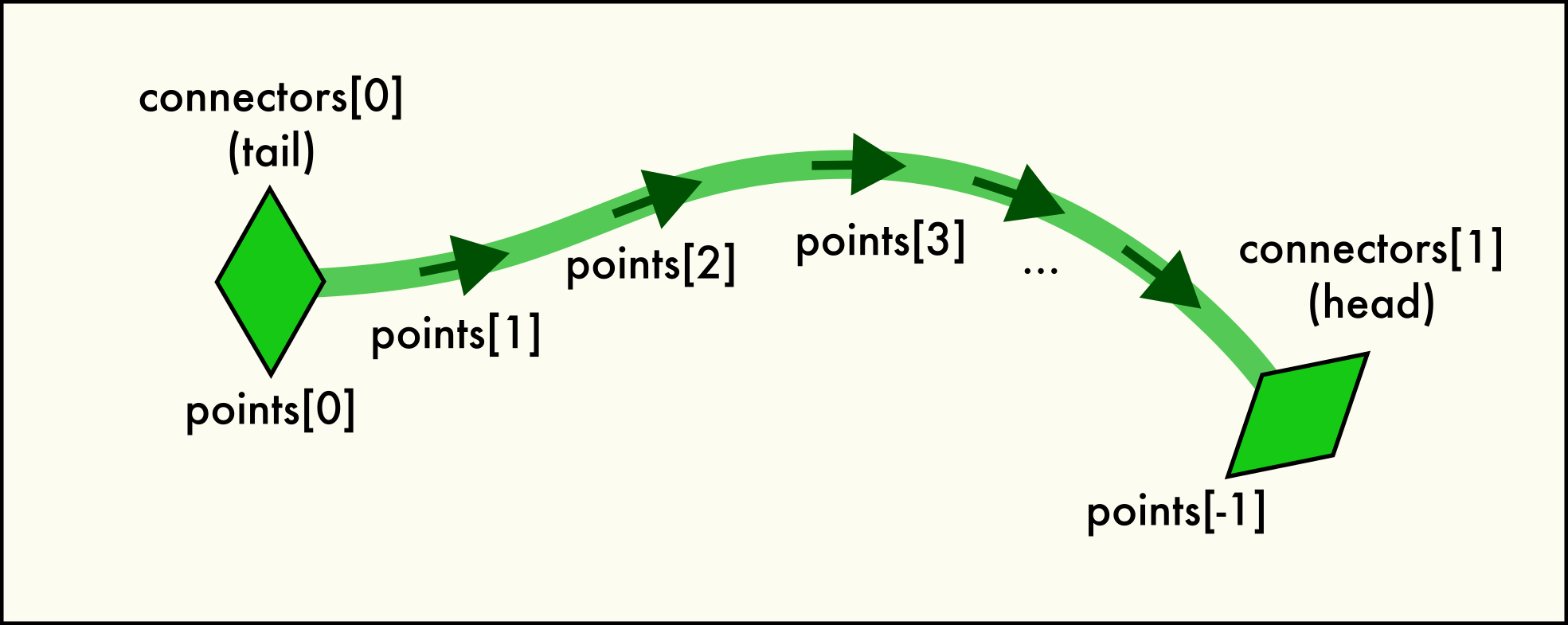
Linehas two end pointconnectorsand is described by a sequence of spatialpoints.A connector object represents one of the two end points of each
Linein the network. In other words, everyLinehas exactly two uniqueConnectorobjects belonging to the line. This pair is accessible via theLine.connectorsattribute. Since dislocations always have a direction (their line sense, with respect to which their Burgers vector is defined), one connector is located at the “head” (forward) and one at the “tail” (backward) end of the directed line.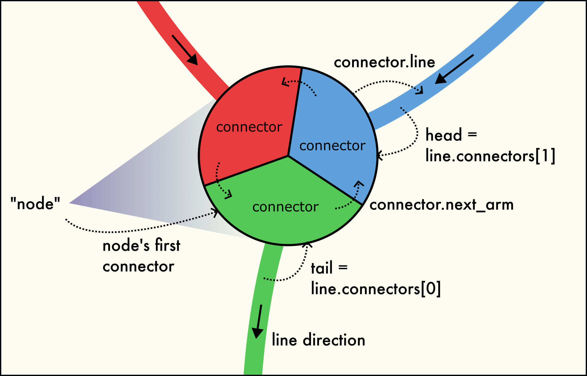
Three dislocation arms meet at a dislocation node (junction). The node is formed by a circular linked-list of connectors.
A dislocation network node (junction) is formed by several connectors located at the same point in space, as illustrated in the figure to the right. This node structure consists of three interlinked connectors belonging to the three dislocation arms meeting in the node. Dislocation arms can be either inbound or outbound.
Network nodes may consist of one, two, three or more connectors:
A single connector, only interlinked with itself, represents a dangling line end. They occur when a dislocation terminates in another extended crystal defect, such as a grain boundary or free surface.
A 2-node, consisting of two interlinked connectors, is part of a dislocation loop or infinite periodic dislocation line. They occur when a dislocation line is closed on itself, i.e, its head and tail are connected.
A node with three or more connectors represents a physical dislocation junction, where three or more arms with non-zero Burgers vector meet.
The connectors belonging to the same network node are interlinked with each other in the form of a circular linked list. The
Connector.next_armfield leads to the next connector in the circular list. The last connector of the node points back to the first connector of the node. This way, all connectors can be visited by starting from any connector of the node and following theConnector.next_armfield until the starting connector is reached again. For a 1-node (a dangling line end), theConnector.next_armfield points to itself.The
Connector.armsmethod yields a list of all connectors belonging to the same local node as this connector (including the connector itself). TheConnector.arm_countproperty counts the number of connectors in the local node. TheConnector.linefield points to theLineobject that the connector belongs to.The
DislocationNetwork.find_nodes()method can be used to generate a list ofConnectorobjects, one for each node in the network. It is useful if you want to iterate over all unique nodes in the network.Added in version 3.10.2.
- property arm_count: int
The number of arms meeting at the node formed by this connector and others, including the connector itself.
- arms() list[Connector]
This method builds a list of
Connectorobjects representing the arms connected to the node. Each connector object links to a different dislocation line incident to the network node.
- property is_head: bool
True if the connector is located at the head of its dislocation line, i.e.,
selfisself.line.connectors[1]. Then the connectedLineis inbound on the node.
- property is_tail: bool
True if the connector is located at the tail of its dislocation line, i.e.,
selfisself.line.connectors[0]. Then the connectedLineis outbound from the node.
- property next_arm: Connector
The
Connectorbelonging to the next dislocation line incident to the node.
- property position: ArrayLike[float64]
The Cartesian coordinates of the connector in the global simulation coordinate system. This corresponds to the start or end point of the dislocation, i.e., either
self.line.points[0]orself.line.points[-1].Note
The positions of the connectors in the same network node are typically identical, but they will differ if their dislocation lines belong to different periodic images of the simulation cell. In this case, the positions of the connectors are shifted by a periodicity vector of the simulation domain.
- class Line
Describes a single continuous dislocation line that is part of a
DislocationNetwork.A dislocation line is a curve in 3d space, approximated by a sequence of
pointsconnected by linear line segments. You can query its total curvelengthor compute some location on the line from a linear path coordinate t using the methodpoint_along_line(). The line is terminated by twoconnectorsat its two end points, which represent the connectivity of the dislocation network.A dislocation line is embedded in some crystallite (a region with uniform lattice orientation), which is identified by the numerical
cluster_id. All dislocation lines belonging to the same crystallite share the same lattice coordinate system in which their true Burgers vectors are expressed. A line’strue_burgers_vectoris given in Bravais lattice units.Each crystallite has a particular mean orientation within the global simulation coordinate system and a mean lattice parameter and elastic strain. Applying these mean crystal properties to the
true_burgers_vectoryields the line’sspatial_burgers_vector, which is expressed in the global coordinate system shared by all dislocations of the entireDislocationNetwork. Thespatial_burgers_vectoris given in simulation coordinate units (typically Angstroms).The
is_loopproperty flag indicates that the two end points of the dislocation line form a 2-junction. This property does not necessarily mean that the dislocation forms an actual circular loop. In simulations using periodic boundary conditions, a straight dislocation can also connect to itself through the periodic cell boundaries and form an infinite periodic line. This situation is indicated by theis_infinite_lineproperty, which implies that theis_loopproperty is also true.All fields of this class are read-only. To modify a dislocation line, you can use the
DislocationNetwork.set_line()method.Changed in version 3.10.2: Renamed this class from
DislocationSegmenttoDislocationNetwork.Line.- property cluster_id: int
The numeric identifier of the crystal cluster containing this dislocation line. A crystal cluster is the technical term for a contiguous group of atoms forming a spatial region with uniform lattice orientation, i.e., a crystallite or grain.
The
true_burgers_vectorof the dislocation is expressed in the local coordinate system of the crystal cluster. Thespatial_burgers_vectorof the dislocation is computed by transforming the true Burgers vector with the mean elastic deformation gradient tensor of the crystal cluster.
- property connectors: tuple[Connector, Connector]
-
A tuple of two
Connectorobjects representing the two end points of the dislocation line. The first connector is located at the start of the line (its tail), the second connector at the end of the line (its head).Added in version 3.10.2.
- property custom_color: tuple[float, float, float]
The RGB color value to be used for visualizing this particular dislocation line, overriding the default coloring scheme imposed by the
DislocationVis.coloring_modesetting. The custom color is only used if its RGB components are non-negative (i.e. in the range 0-1); otherwise the line will be rendered using the computed color depending on the line’s Burgers vector.- Default:
(-1.0, -1.0, -1.0)
- property id: int
The unique numerical identifier of this dislocation line within the
DislocationNetwork. This is simply the zero-based index of the line in theDislocationNetwork.lineslist.Important: This identifier is derived from the arbitrary storage order of the lines in the network and cannot be used to identify the same dislocation in another simulation snapshot.
- property is_infinite_line: bool
Indicates that this dislocation is an infinite line passing through a periodic simulation box boundary. A dislocation is considered infinite if it is a closed loop but its start and end do not coincide (because they are located in different periodic images).
- property is_loop: bool
Indicates whether this line forms a loop, i.e., its end is connected to its start point. Note that an infinite dislocation line passing through a periodic simulation cell boundary is also considered a logical loop (see
is_infinite_lineproperty).
- property length: float
Computes the length of this dislocation line in simulation units of length, integrating the piecewise linear segments it is made of.
- point_along_line(t: float) NDArray[float64]
Returns the Cartesian coordinates of a point on the dislocation line. The location to be calculated must be specified in the form of a fractional position t along the continuous dislocation line.
- Parameters:
t – Normalized path coordinate in the range [0,1]
- Returns:
The xyz coordinates of the requested point on the dislocation line.
Added in version 3.10.0.
- property points: NDArray[float64]
The sequence of spatial points that define the curved shape of this dislocation (in simulation coordinates). This is a N x 3 Numpy array, with N>2 being the number of points along the line.
For true dislocation loops, the first and the last point in the list coincide exactly. For infinite lines, the first and the last point coincide modulo a periodicity vector of the simulation domain.
The point sequence always forms a continuous line, which may lead outside the primary
SimulationCellif periodic boundary conditions (PBCs) are used, i.e., only the start of the dislocation is always inside the primary simulation cell but its end point may not. Thus, the line is stored in unwrapped form. A wrapping happens ad-hoc during visualization, when theDislocationViselement renders the dislocation network or if the network is exported to a file format, e.g. VTK, which does not support PBCs.
- property spatial_burgers_vector: NDArray[float64]
The Burgers vector of the segment, expressed in the global coordinate system of the simulation. This vector is calculated by transforming the true Burgers vector from the local lattice coordinate system to the global simulation coordinate system using the average orientation matrix of the crystal cluster the dislocation segment is embedded in.
- property true_burgers_vector: NDArray[float32]
The Burgers vector of the dislocation expressed in the local coordinate system of the crystal the dislocation is located in. The true Burgers vectors of two dislocation lines may only be added if both belong to the same
cluster_id.
- find_nodes() list[Connector]
Returns a list of all unique dislocation nodes in the network, each represented by a
Connector.For a detailed description of what a “node” is, see the
Connectorclass. The list returned by this method contains one (arbitrary)Connectorfrom each network node, in no particular order. Each of these connectors serves as access into a node and can be used to visit the other connectors (dislocation arms) in the same node viaConnector.arms:network = data.dislocations for node in network.find_nodes(): print(node.arm_count, node.position) for arm in node.arms(): print(arm.line.true_burgers_vector)
Added in version 3.10.2.
- property lines: Sequence[Line]
The list of dislocation lines in this dislocation network. This list-like object contains
Lineobjects in arbitrary order and is read-only.
- set_line(index: int, true_burgers_vector: ArrayLike | None = None, cluster_id: int | None = None, points: ArrayLike | None = None, custom_color: ArrayLike | None = None)
This method can be used to manipulate certain aspects of a
Linein the network. Fields for which no new value is specified will keep their current values.- Parameters:
index – The zero-based index of the dislocation line to modify in the
linesarray.true_burgers_vector – The new lattice-space Burgers vector (
true_burgers_vector).cluster_id – The numeric ID of the crystallite cluster the dislocation line is embedded in (
cluster_id).points – An \((N, 3)\) NumPy array of Cartesian coordinates containing the dislocation’s vertices (
points).custom_color – RGB color to be used for rendering the line instead of the automatically determined color (
custom_color).
Example of a user-defined modifier function that manipulates the dislocation line data:
import numpy as np

def modify(frame: int, data: DataCollection):

    # Flip Burgers vector and line sense of each dislocation:
    for index, line in enumerate(data.dislocations.lines):
        data.dislocations_.set_line(index,
            true_burgers_vector = np.negative(line.true_burgers_vector),
            points = np.flipud(line.points))

    # Highlight all 1/6[121] dislocations by giving them a red color:
    for index, line in enumerate(data.dislocations.lines):
        if np.allclose(line.true_burgers_vector, (1/6, 2/6, 1/6)):
            data.dislocations_.set_line(index, custom_color=(1, 0, 0))
- class ovito.data.ElementType
Base:
ovito.data.DataObjectThis class describes a single “type”, for example a particle or bond type, that is part of a typed property array.
The
ElementTypeclass is the generic base class used for all type descriptors in OVITO. It stores general attributes such as a type’s unique numericid, its human-readablename, and its displaycolor. Note that, for certain typed properties, OVITO uses more specific sub-classes such asParticleTypeandBondType, which can store additional attributes such asradiusandmass.The
ElementTypeinstances associated with a typed property are found in theProperty.typeslist.You can use the
Property.type_by_id()andProperty.type_by_name()methods to look up a certainElementTypebased on a numeric identifier or name string.- property color: tuple[float, float, float]
The color used when rendering elements of this type. This is a RGB tuple with components in the range 0.0 – 1.0.
- Default:
(1.0, 1.0, 1.0)
- property enabled: bool
Controls whether this type is currently active or inactive. This flag currently has a meaning only in the context of atomic structure identification. Some analysis modifiers manage a list of the structure types they can identify (e.g. FCC, BCC, etc.). The identification of individual structure types can be turned on or off by the user by changing their
enabledflag. SeeStructureIdentificationModifier.structuresfor further information.- Default:
True
- property id: int
The unique numeric identifier of the type (typically some positive
int). The identifier is and must be unique among all element types in thetypeslist of a typedProperty. Thus, if you create a new element type, make sure you give it a unique id before inserting it into thetypeslist of a typed property.- Default:
0
- class ovito.data.Lines
Base:
ovito.data.PropertyContainerAdded in version 3.10.0.
The
Linesclass represents one or more 3D polylines. You can create an instance of this class in aDataCollectionusing theGenerateTrajectoryLinesModifieror theDataCollection.lines.create()method.You can retrieve existing
Linesobjects from a pipeline’s output through theDataCollection.linesdictionary view. EachLinesobject has a uniqueidentifiername that serves as a lookup key.Linesobjects are always associated withLinesViselement, which controls the visual appearance of the lines in rendered images. You can access the visual element through thevisattribute provided by theDataObjectbase class. TheLinesViselement provides the capability to visualize a local quantity defined at each line vertex using pseudo-color mapping.The
Linescontainer uses the following standard properties with predefined names and data layouts. Additional per-vertex properties may be added using thecreate_property()method of the base class.Property name
Python access
Data type
Component names
Color
float32
R, G, B
Position
float64
X, Y, Z
Section
int64
Selection
int8
Time
int32
Data model
The
Linesdata object type isPropertyContainer, which means it consist of a set of uniform property arrays. The standard property Position stores the vertex coordinates. When rendering aLinesobject, consecutive vertices get connected by linear line segments to form a polyline (which is also called a line “section”). To denote the end of a contiguous polyline and the start of a new one, the property Section must be filled with section identifiers, which mark consecutive sequences of vertices, each forming a separate polyline. Section identifiers are arbitrary integer numbers that stay the same within a polyline but change from one polyline to the next:
Example: Definition of three polylines of length 2, 3, and 2, respectively. Vertex
Position
Section
0
\((x_0, y_0, z_0)\)
0
1
\((x_1, y_1, z_1)\)
0
2
\((x_2, y_2, z_2)\)
1
3
\((x_3, y_3, z_3)\)
1
4
\((x_4, y_4, z_4)\)
1
5
\((x_5, y_5, z_5)\)
2
6
\((x_6, y_6, z_6)\)
2
The
Linesclass provides thecreate_line()method to add new polylines to the container. It appends a list of vertex coordinates to the Position property and automatically assigns a new unique Section value to these vertices to define a new polyline.Note
In a
Linesobject created by theGenerateTrajectoryLinesModifier, the Section property reflects the unique identifiers of the particles that traced the individual trajectory lines.If the Time property is present, it stores the animation frame number at which each vertex should appear in a trajectory animation. This feature allows to animate the lines over time and is used for particle trajectory visualization. The gradual rendering of lines is only active if the
LinesVis.upto_current_timeoption is enabled in the attached visual element.- property colors: Property | None
The
Propertydata array for the Color standard (line property); orNoneif that property is undefined.
- create_line(positions)
Adds a new section (a polyline) to an existing
Linescontainer. The container’s vertexcountwill be incremented by the number of newly inserted points. The method copies positions into thePositionproperty array after extending the array and gives the new polyline a uniqueSectionproperty value.
- property positions: Property | None
The
Propertyarray containing the XYZ coordinates of the line vertices (standard property Position). May beNoneif the property is not defined yet. Usecreate_property()to add the property to the container if necessary. Usepositions_(with an underscore) to access an independent copy of the array, whose contents can be safely modified in place.
- property sections: Property | None
The
Propertyarray with the section each line vertex belongs to (standard property Section). May beNoneif the property is not defined yet. Usecreate_property()to add the property to the container if necessary. Usesections_(with an underscore) to access an independent copy of the array, whose contents can be safely modified in place.
- property selection: Property | None
The
Propertydata array for theSelectionstandard line vertices property; orNoneif that property is undefined.
- property time_stamps: Property | None
The
Propertyarray with the time stamps of the line vertices (standard property Time). May beNoneif the property is not defined yet. Usecreate_property()to add the property to the container if necessary. Usetime_stamps_(with an underscore) to access an independent copy of the array, whose contents can be safely modified in place.
- class ovito.data.NearestNeighborFinder(N, data_collection)
A utility class that finds the N nearest neighbors of a particle or around some other spatial query point.
See also
To find all neighbors within a spherical cutoff region around another particle, use the
CutoffNeighborFinderinstead.The class constructor takes the requested number of nearest neighbors, N, and a
DataCollectioncontaining the input particles and the optional simulation cell. N must be a positive integer not greater than 64, which is the maximum number of neighbors supported by this class.Note
Keep in mind that, if the system contains only N particles or less, and if the simulation cell does not use periodic boundary conditions, then the search algorithm will return less than the requested number of nearest neighbors.
Once the
NearestNeighborFinderhas been initialized, you can call itsfind()method to iterate over the sorted list of nearest neighbors of a given central particle:# Set up a neighbor finder for visiting the 12 closest neighbors of each particle. finder = NearestNeighborFinder(12, data) # Loop over all input particles: for index in range(data.particles.count): print("Nearest neighbors of particle %i:" % index) # Iterate over the neighbors of the current particle, starting with the closest: for neigh in finder.find(index): print(neigh.index, neigh.distance, neigh.delta) # The index can be used to access properties of the current neighbor, e.g. type_of_neighbor = data.particles.particle_types[neigh.index]
In addition, the class provides the
find_at()method, which determines the N nearest particles around some arbitrary spatial location:# Visit particles closest to some spatial point (x,y,z): xyz_coords = (0.0, 0.0, 0.0) for neigh in finder.find_at(xyz_coords): print(neigh.index, neigh.distance, neigh.delta)
The corresponding
find_all()andfind_all_at()methods allow you to perform these queries efficiently for multiple particles or spatial locations at once.- find(index)
Returns an iterator that visits the N nearest neighbors of the given particle in order of ascending distance.
- Parameters:
index (int) – The zero-based index of the central particle whose neighbors should be determined.
- Returns:
A Python iterator that visits the N nearest neighbors of the central particle in order of ascending distance. For each neighbor being visited, the iterator returns an object having the following attributes:
index: The global index of the current neighbor particle.
distance: The distance of the current neighbor from the central particle.
distance_squared: The squared neighbor distance.
delta: The three-dimensional vector connecting the central particle with the current neighbor (correctly taking into account periodic boundary conditions).
- Return type:
The index can be used to look up properties of the neighbor particle, as demonstrated in the first example code above.
Note that several periodic images of the same particle may be visited if the periodic simulation cell is sufficiently small. Then the same particle index will appear more than once in the neighbor list. In fact, the central particle may be among its own neighbors in a sufficiently small periodic simulation cell. However, the computed neighbor vector (delta) will be unique for each image of a neighboring particle.
The number of neighbors actually visited may be smaller than the requested number, N, if the system contains too few particles and is non-periodic.
Note that the
find()method will not find other particles located exactly at the same spatial position as the central particle for technical reasons. To find such particles too, which are positioned exactly on top of each other, usefind_at()instead.
- find_all(indices=None)
Finds the N nearest neighbors of each particle in the system or of the subset of particles specified by indices. This is the batch-processing version of
find(), allowing you to efficiently compute the neighbor lists and neighbor vectors of several particles at once, without explicit for-loop and by making parallel use of all available processor cores.- Parameters:
indices (Optional[ArrayLike]) – List of zero-based particle indices for which the neighbor lists should be computed. If left unspecified, neighbor lists will be computed for every particle in the system.
- Returns:
(neigh_idx, neigh_vec)- Return type:
The method returns two arrays:
neigh_idx: NumPy array of shape (M, N) storing the indices of neighbor particles, with M equal to len(indices) or, if indices is None, the total number of particles in the system. N refers to the number of nearest neighbors requested in theNearestNeighborFinderconstructor. The computed indices in this array can be used to look up properties of neighbor particles in the globalParticlesobject.neigh_vec: NumPy array of shape (M, N, 3) storing the xyz components of the three-dimensional neighbor vectors (“delta”), which connect the M central particles with their N respective nearest neighbors.Tip
To compute all pair-wise distances in one go, i.e. the 2-norms of the neighbor vectors, you can do:
distances = numpy.linalg.norm(neigh_vec, axis=2) # Yields (M,N) array of neighbor distances
- find_all_at(coords)
Finds the N nearest neighbors around each spatial point specified by coords. This is the batch-processing version of
find_at(), allowing you to efficiently determine the closest neighbors around several spatial locations at once, without an explicit for-loop and by making parallel use of all available processor cores.- Parameters:
coords (ArrayLike) – NumPy array of shape (M, 3) containing the xyz coordinates of M query points at each of which the N nearest particles should be found.
- Returns:
(neigh_idx, neigh_vec)- Return type:
The method returns two NumPy arrays:
neigh_idx: NumPy array of shape (M, N) storing the indices of nearest particles, with M equal to len(coords). N refers to the number of nearest neighbors requested in theNearestNeighborFinderconstructor. Each neighbor list is sorted by distance from the corresponding query point.neigh_vec: NumPy array of shape (M, N, 3) storing the xyz components of the three-dimensional neighbor vectors (“delta”), which connect the M query points with their N respective nearest neighbors.If there is a particle located exactly at a query location, it will be among the returned neighbors for that point. This is in contrast to the
find_all()function, which skips the central particles at the query locations.The number of returned neighbors may be smaller than the requested number, N, if the system contains fewer than N particles and is non-periodic. In this case, the corresponding columns of
neigh_idxwill be filled up with -1.Added in version 3.11.0.
- find_at(coords)
Returns an iterator that visits the N nearest particles around a spatial point given by coords in order of ascending distance. Unlike the
find()method, which queries the nearest neighbors of a physical particle,find_at()allows searching for nearby particles at arbitrary locations in space.- Parameters:
coords (ArrayLike) – A coordinate triplet (x,y,z) specifying the spatial location where the N nearest particles should be queried.
- Returns:
A Python iterator that visits the N nearest neighbors in order of ascending distance. For each visited particle the iterator returns an object with the following attributes:
index: The index of the current particle (starting at 0).
distance: The distance of the current neighbor from the query location.
distance_squared: The squared distance to the query location.
delta: The three-dimensional vector from the query point to the current particle (correctly taking into account periodic boundary conditions).
- Return type:
If there is a particle located exactly at the query location coords, it will be among the returned neighbors. This is in contrast to the
find()function, which skips the central particle itself.The number of neighbors actually visited may be smaller than the requested number, N, if the system contains too few particles and is non-periodic.
- class ovito.data.ParticleType
Base:
ovito.data.ElementTypeThis data object describes one particle or atom type. In atomistic simulations, each chemical element is typically represented by an instance of the
ParticleTypeclass. The attributes of this class control how the particles of that type get visualized in terms of e.g. color, particle radius, shape, etc.The
ParticleTypeclass inherits several general attribute fields from its base classElementType, e.g. thecolor,nameandidfields. It adds specific fields for particles:radiusandshape. Furthermore, the class has additional fields controlling the visual appearance of particles with user-defined shapes.The
ParticleTypeinstances all live in theProperty.typeslist of the'Particle Type'standardPropertyarray, which is accessible asParticles.particle_types. The association of particles with particle types is established through the unique type IDs. The following code shows how to first list all unique particle types defined for a structure and then print each particle’s type ID by iterating over the data array:# Access the property with the name 'Particle Type': type_property = data.particles.particle_types # Print list of particle types (their numeric IDs and names) for t in type_property.types: print(f'ID {t.id} -> {t.name}') # Print the numeric type ID of each particle: for tid in type_property[...]: print(tid)
A common task is to look up the
ParticleTypethat corresponds to a given numeric type ID. For this, thePropertyclass provides thetype_by_id()method:# Look up the particle type with unique ID 2: t = type_property.type_by_id(2) print(t.name, t.color, t.radius) # Iterate over all particles and print their type's name: for tid in type_property[...]: print(type_property.type_by_id(tid).name)
Another common operation is to look up a particle type by name, for example the type representing a certain chemical element. For this type of look-up the
type_by_name()method is available, which assumes that types have uniquenames:print(type_property.type_by_name('Si').id) # Print numeric ID of type 'Si'
- property backface_culling: bool
Activates back-face culling for the user-defined particle shape mesh to speed up rendering. If turned on, polygonal sides of the shape mesh facing away from the viewer will not be rendered. You can turn this option off if the particle’s shape is not closed and two-sided rendering is required. This option only has an effect if a user-defined shape has been assigned to the particle type using the
load_shape()method.- Default:
True
- property highlight_edges: bool
Activates the highlighting of the polygonal edges of the user-defined particle shape during rendering. This option only has an effect if a user-defined shape has been assigned to the particle type using the
load_shape()method.- Default:
False
- load_defaults()
Given the type’s chemical
name, which must have been set before invoking this method, initializes the type’scolor,radius,vdw_radiusandmassfields with default values from OVITO’s internal database of chemical elements.See also
- load_shape(filepath: str)
Assigns a user-defined shape to the particle type. Particles of this type will subsequently be rendered using the polyhedral
meshloaded from the given file. The method will automatically detect the format of the geometry file and supports standard file formats such as OBJ, STL and VTK that contain triangle meshes, see this table.The shape loaded from the geometry file will be scaled with the
radiusvalue set for this particle type or the per-particle value stored in theRadiusparticle property if present. The shape of each particle will be rendered such that its origin is located at the coordinates of the particle (Positionproperty).The following example script demonstrates how to load a user-defined shape for the first particle type (index 0) loaded from a LAMMPS dump file, which can be accessed through the
Property.typeslist of theParticle Typeparticle property.pipeline = import_file("input/simulation.dump") pipeline.add_to_scene() types = pipeline.source.data.particles_.particle_types_ types.type_by_id_(1).load_shape("input/tetrahedron.vtk") types.type_by_id_(1).highlight_edges = True
- property mesh: TriangleMesh | None
The
TriangleMeshobject to be used as custom shape for rendering particles of this type. You can either programmatically create aTriangleMeshfrom a list of vertices and faces and assign it to this field, or let theload_shape()method read the shape mesh from a separate geometry file. Also some file readers (e.g. GSD and Aspherix) may generate the shape mesh automatically based on information found in the simulation file.The
ParticlesViselement, which is responsible for visualizing a particle system, will render an instance of the mesh at each particle site, uniformly scaled by the particle’sradius, translated by the coordinates taken from thePositionparticle property, and rotated by the quaternion transformation taken from theOrientationparticle property.Note: This mesh will be ignored by the
ParticlesViselement unless the type’sshapeis set toParticlesVis.Shape.Mesh.- Default:
None
Added in version 3.8.0.
- property radius: float
This attribute controls the display radius of all particles of this type.
When set to zero, particles of this type will be rendered using the standard size specified by the
ParticlesVis.radiusparameter. Furthermore, precedence is given to any per-particle sizes assigned to theRadiusparticle property if that property has been defined.- Default:
0.0
The following example script demonstrates how to set the display radii of two particle types loaded from a simulation file, which can be accessed through the
Property.typeslist of theParticle Typeparticle property.pipeline = import_file("input/simulation.dump") pipeline.add_to_scene() def setup_particle_types(frame, data): types = data.particles_.particle_types_ types.type_by_id_(1).name = "Cu" types.type_by_id_(1).radius = 1.35 types.type_by_id_(2).name = "Zr" types.type_by_id_(2).radius = 1.55 pipeline.modifiers.append(setup_particle_types)
- property shape: ParticlesVis.Shape
Selects the geometric shape used when rendering particles of this type. Supported modes are:
ParticlesVis.Shape.Unspecified(default)ParticlesVis.Shape.SphereParticlesVis.Shape.BoxParticlesVis.Shape.CircleParticlesVis.Shape.SquareParticlesVis.Shape.CylinderParticlesVis.Shape.SpherocylinderParticlesVis.Shape.Mesh
By default, the standard particle shape that is set in the
ParticlesVisvisual element is used to render particles of this type. Parameter values other thanUnspecifiedallow you to control the rendering shape on a per-type basis. ModeSphereincludes ellipsoid and superquadric particle shapes, which are enabled by the presence of theAspherical ShapeandSuperquadric Roundnessparticle properties.The
load_shape()method lets you specify a user-definedmeshgeometry for this particle type. Calling this method automatically switches the shape parameter to modeMesh.Setting the shapes of particle types permanently, i.e., for all frames of a loaded simulation trajectory, typically requires a user-defined modifier function. This function is inserted into the
Pipelineto make the necessary changes to theParticleTypeobjects associated with thePropertynamedParticle Type:from ovito.io import import_file from ovito.vis import * # Load a simulation file containing numeric particle types 1, 2, 3, ... pipeline = import_file("input/nylon.data") pipeline.add_to_scene() # Set the default particle shape in the ParticlesVis visual element, # which will be used by all particle types for which we do not specify a different shape below. pipeline.compute().particles.vis.shape = ParticlesVis.Shape.Box pipeline.compute().particles.vis.radius = 1.0 # A user-defined modifier function that configures the shapes of particle types 1 and 2: def setup_particle_types(frame, data): # Write access to property 'Particle Type': types = data.particles_.particle_types_ # Write access to numeric ParticleTypes, which are sub-objects of the Property object: types.type_by_id_(1).radius = 0.5 types.type_by_id_(1).shape = ParticlesVis.Shape.Cylinder types.type_by_id_(2).radius = 1.2 types.type_by_id_(2).shape = ParticlesVis.Shape.Sphere pipeline.modifiers.append(setup_particle_types) # Render a picture of the 3d scene: vp = Viewport(camera_dir = (-2,1,-1)) vp.zoom_all() vp.render_image(filename='output/particles.png', size=(320,240), renderer=TachyonRenderer())
- property use_mesh_color: bool
Use the intrinsic mesh color(s) instead of the particle color when rendering particles of this type. This option only has an effect if a user-defined shape
meshhas been assigned to this particle type, e.g., by calling theload_shape()method.- Default:
False
- property vdw_radius: float
The van der Waals radius of the particle type. This value is used by the
CreateBondsModifierto decide which pairs of particles are close enough to be connected by a bond. In contrast to theradiusparameter, the van der Waals radius does not affect the visual appearance of the particles of this type.- Default:
0.0
- class ovito.data.Particles
Base:
ovito.data.PropertyContainerThis object stores a system of particles and their properties. Additional things which are typically associated with molecular systems, e.g.
bonds,angles, etc. are stored in corresponding sub-objects.A
Particlesobject is usually part of aDataCollectionwhere it can be found via theDataCollection.particlesproperty.The total number of particles is specified by the
countattribute, which theParticlesclass inherits from itsPropertyContainerbase class.Particles are usually associated with a set of properties, e.g. position, type, velocity. Each of the properties is represented by a separate
Propertydata object, which is basically an array of numeric values, one for each particle in the system. A particle property is identified by its unique name and can be looked up via the dictionary interface of thePropertyContainerbase class. OVITO predefines a set of standard properties, which have a fixed data layout, meaning, and role:Standard property name
Data type
Component names
Angular Momentum
float64
X, Y, Z
Angular Velocity
float64
X, Y, Z
Aspherical Shape
float32
X, Y, Z
Centrosymmetry
float64
Charge
float64
Cluster
int64
Color
float32
R, G, B
Coordination
int32
Deformation Gradient
float64
XX, YX, ZX, XY, YY, ZY, XZ, YZ, ZZ
Dipole Magnitude
float64
Dipole Orientation
float64
X, Y, Z
Displacement Magnitude
float64
Displacement
float64
X, Y, Z
DNA Strand
int32
Elastic Deformation Gradient
float64
XX, YX, ZX, XY, YY, ZY, XZ, YZ, ZZ
Elastic Strain
float64
XX, YY, ZZ, XY, XZ, YZ
Force
float64
X, Y, Z
Kinetic Energy
float64
Mass
float64
Molecule Identifier
int64
Molecule Type
int32
Nucleobase
int32
Nucleotide Axis
float64
X, Y, Z
Nucleotide Normal
float64
X, Y, Z
Orientation
float32
X, Y, Z, W
Particle Identifier
int64
Particle Type
int32
Periodic Image
int32
X, Y, Z
Position
float64
X, Y, Z
Potential Energy
float64
Radius
float32
Rotation
float64
X, Y, Z, W
Selection
int8
Spin
float64
Strain Tensor
float64
XX, YY, ZZ, XY, XZ, YZ
Stress Tensor
float64
XX, YY, ZZ, XY, XZ, YZ
Stretch Tensor
float64
XX, YY, ZZ, XY, XZ, YZ
Structure Type
int32
Superquadric Roundness
float32
Phi, Theta
Torque
float64
X, Y, Z
Total Energy
float64
Transparency
float32
Vector Color
float32
R, G, B
Vector Transparency
float32
Velocity Magnitude
float64
Velocity
float64
X, Y, Z
For some of the most important properties, this container class provides quick access getters such as
positions,identifiers, orparticle_typesto look them up:coords = data.particles.positions
User-defined particle properties having non-standard names, and standard properties for which no quick access getter exists, can be looked up by literal name:
mol_ids = data.particles['Molecule Identifier']
For more information on how to add or modify particle properties, please see the
PropertyContainerandPropertyclasses.- add_particle(position)
Adds a new particle to the model. The particle
countwill be incremented by one. The method assigns position to thePositionproperty of the new particle. The values of all other properties are initialized to zero.- Parameters:
position (ArrayLike) – The xyz coordinates for the new particle.
- Returns:
The 0-based index of the newly created particle, which is
(Particles.count-1).- Return type:
- property angles: PropertyContainer | None
A
PropertyContainerstoring the list of angles defined for the molecular model (may beNone).
- property bonds: Bonds | None
The
Bondsdata object storing the list of bonds and their properties (may beNone).
- property colors: Property | None
The
Propertydata array for theColorstandard particle property; orNoneif that property is undefined.
- create_bonds(*, vis_params=None, **params)
This convenience method conditionally creates and associates a
Bondsobject with thisParticlesparent object. If there is already an existing bonds object (bondsis notNone), then that bonds object is replaced with a modifiable copy if necessary. The attachedBondsViselement is preserved.- Parameters:
params (Any) – Key-value pairs passed to the method as keyword arguments are used to set attributes of the
Bondsobject (even if the bonds object already existed).vis_params (Mapping[str, Any] | None) – Optional dictionary to initialize attributes of the attached
BondsViselement (only used if the bonds object is newly created by the method).
- Return type:
The logic of this method is roughly equivalent to the following code:
def create_bonds(particles: Particles, vis_params=None, **params) -> Bonds:
    if particles.bonds is None:
        particles.bonds = Bonds()
        if vis_params:
            for name, value in vis_params.items(): setattr(particles.bonds.vis, name, value)
    for name, value in params.items(): setattr(particles.bonds_, name, value)
    return particles.bonds_
Usage example:
pairs = [(0, 1), (1, 2), (2, 0)] # Pairs of particle indices to connect by bonds
bonds = data.particles_.create_bonds(count=len(pairs), vis_params={'width': 0.6})
bonds.create_property('Topology', data=pairs)
Added in version 3.7.4.
- delta_vector(a, b, cell, return_pbcvec=False)
Computes the vector connecting two particles a and b in a periodic simulation cell by applying the minimum image convention.
This is a convenience wrapper for the
SimulationCell.delta_vector()method, which computes the vector between two arbitrary spatial locations \(r_a\) and \(r_b\) taking into account periodic boundary conditions. The version of the method described here takes two particle indices a and b as input, computing the shortest vector \({\Delta} = (r_b - r_a)\) between them using the minimum image convention. Please see theSimulationCell.delta_vector()method for further information.- Parameters:
a (int | Sequence[int]) – Zero-based index of the first input particle. This may also be an array of particle indices.
b (int | Sequence[int]) – Zero-based index of the second input particle. This may also be an array of particle indices with the same length as a.
cell (SimulationCell) – The periodic domain. Typically,
DataCollection.cellis used as argument here.return_pbcvec (bool) – If true, lets the method also return the vector \(n\), which specifies how often the computed particle-to-particle vector crosses the cell’s face.
- Returns:
The delta vector and, optionally, the vector \(n\).
- Return type:
- property dihedrals: PropertyContainer | None
A
PropertyContainerstoring the list of dihedrals defined for the molecular model (may beNone).
- property forces: Property | None
The
Propertydata array for theForcestandard particle property; orNoneif that property is undefined.
- property identifiers: Property | None
Returns a
Propertydata array containing the values of theParticle Identifierstandard particle property; orNoneif that particle property does not exist.The property array stores the numerical IDs that are typically used by simulation codes to uniquely identify individual particles.
Note
A particle identifier is an arbitrary and unique 64-bit integer value permanently associated with a particle. In contrast, the particle’s index is implicitly given by the particle’s current position within the particles list.
If you delete some of the particles from the system, using the
DeleteSelectedModifieror thedelete_elements()method for example, the indices of the remaining particles get typically shifted but their unique IDs stay the same.Some of OVITO’s simulation file readers provide the option to sort the list of particles by ID during import to obtain a stable ordering. Generally, however, the storage order of particles is arbitrary and can vary between frames of a trajectory. The
remap_indices()method can be useful in this situation.Note
The value of
identifiersmay beNone, which means particles don’t have any identifiers. Many operations in OVITO then assume that the ordering and total count of particles are constant throughout the entire simulation trajectory and the identities are implicitly given by the particles’ indices.Given some list of zero-based particle indices, determining the corresponding unique identifiers requires just a simple NumPy indexing expression:
query_indices = [0, 7, 3, 2] # <-- zero-based particle indices for which we want to look up IDs
ids = data.particles.identifiers[query_indices]
assert len(ids) == len(query_indices)
The reverse lookup, i.e., finding the indices at which particles with certain IDs are stored in the list, requires some more work. That’s because particles may be stored in arbitrary order, i.e., the sequence of unique IDs is generally not sorted nor contiguous. A rather slow approach is to
searchthrough the entire array of IDs to locate the one we are looking for:query_id = 37 # <-- a unique particle ID we are looking for index = numpy.argwhere(data.particles.identifiers == query_id)[0,0] assert data.particles.identifiers[index] == query_id
We can speed things up with some extra effort, which pays off when there is a need to look up several particle IDs. To this end, we first
sortthe list of IDs, then perform a more efficientsorted search, and finally map the found indices back to the original particle ordering:query_ids = [2, 37, 8] # <-- some unique particle IDs we want to look up all at once ordering = numpy.argsort(data.particles.identifiers) indices = ordering[numpy.searchsorted(data.particles.identifiers, query_ids, sorter=ordering)] assert numpy.array_equal(data.particles.identifiers[indices], query_ids)
The above
assertstatements are for illustration purposes only.
- property impropers: PropertyContainer | None
A
PropertyContainerstoring the list of impropers defined for the molecular model (may beNone).
- property masses: Property | None
The
Propertydata array for theMassstandard particle property; orNoneif that property is undefined.
- property orientations: Property | None
The
Propertydata array for theOrientationstandard particle property; orNoneif that property is undefined.
- property particle_types: Property | None
The
Propertydata array for theParticle Typestandard particle property; orNoneif that property is undefined.
- property positions: Property | None
Returns the
Propertydata array storing the particle coordinates, i.e. the values of thePositionstandard particle property. Accessing this field is equivalent to a name-based lookup in thePropertyContainer:assert data.particles.positions is (data.particles['Position'] if 'Position' in data.particles else None)
Under special circumstances the
Positionparticle property might not be defined (yet). Then the value isNone.Note
The returned
Propertywill likely be write-protected. If you intend to modify (some of) the particle coordinates in the property array, request a modifiable version of the array by using the underscore notation:data.particles_.positions_[:] = new_coordinates
Alternatively, you can use the
create_property()method to newly create or overwrite the entire property:data.particles_.create_property('Position', data=new_coordinates)
- remap_indices(particles: Particles, indices: Sequence[int] = None) ndarray | slice
In case the storage order of atoms or particles changes during the course of a simulation, this method can determine the mapping of particles from one snapshot of the trajectory to another. It uses the unique
identifiersof the particles to do that.Given two data collections A and B containing the same set of particles but in different order,
remap_indices()determines for each particle in B the zero-based index at which the same particle is found in A. For instance:>>> A = pipeline.compute(frame=0) >>> B = pipeline.compute(frame=1) >>> A.particles.identifiers[...] [8 101 5 30 99] >>> B.particles.identifiers[...] [5 101 30 99 8] >>> A.particles.remap_indices(B.particles) [2 1 3 4 0]
The index mapping generated by
remap_indices()allows you to retrieve property values of particles in A in the same order in which they appear in B, making it easy to perform computations involving property values at different trajectory timesteps, e.g.:mapping = A.particles.remap_indices(B.particles) displacements = B.particles.positions - A.particles.positions[mapping]
remap_indices()compares the uniqueidentifiersstored in theParticle Identifierproperty arrays of both snapshots to compute the index permutation map. If this property is not defined, which may be the case if the imported trajectory file did not contain atom IDs, theremap_indices()method simply assumes that both snapshots use the same constant storage order and returns the identity mapping - as a Pythonsliceobject for optimal performance when being used for NumPy indexing. A slice object is also returned in case the ordering of particle IDs turns out to be the same in both snapshots and no remapping is necessary.Note
An error will be raised if particles with duplicate IDs occur in snapshot A - but it is okay if B contains duplicate IDs. Furthermore, it is not an error if A contains additional particles that are not present in B - as long as all particles from B are found in A.
The default behavior of the method is to look up all particles of B in A. But the index mapping can also be established just for a subset of particles from B by supplying the optional parameter indices. The method expects an array of zero-based indices specifying which particles from snapshot B should be looked up in snapshot A. The returned mapping will have the same length as indices. Example:
# The numeric ID of atom type 'H':
hydrogen_type = B.particles.particle_types.type_by_name('H').id
# Determine the indices of all H atoms in data collection B:
hydrogen_indices = numpy.flatnonzero(B.particles.particle_types == hydrogen_type)

# Determine the corresponding indices of the same atoms in data collection A:
mapping = A.particles.remap_indices(B.particles, hydrogen_indices)

# In snapshot A the same particles are all H atoms too:
assert numpy.all(A.particles.particle_types[mapping] == hydrogen_type)
Added in version 3.7.5.
- property selection: Property | None
The
Propertydata array for theSelectionstandard particle property; orNoneif that property is undefined.
- property structure_types: Property | None
The
Propertydata array for theStructure Typestandard particle property; orNoneif that property is undefined.
- property velocities: Property | None
The
Propertydata array for theVelocitystandard particle property; orNoneif that property is undefined.
- class ovito.data.Property
Base:
ovito.data.DataObjectA storage array for the values of one uniform property of particles, bonds, voxel grid cells, etc. For example, the “Position” property of particles is represented by one
Propertyobject storing the xyz coordinates of all the particles.Propertyobjects are always managed by a specific sub-type of thePropertyContainerclass, for exampleParticles,Bonds,VoxelGrid, orDataTable. These container classes allow to add and remove properties to the data elements they represent. The properties within thePropertyContainerare accessed by name. Here, for example, the particle property holding the particle coordinates:positions = data.particles['Position']
This
Propertyobject behaves almost like a regular NumPy array. For example, you can access the value for the i-th element using array indexing:print('XYZ coordinates of first particle:', positions[0]) print('z-coordinate of sixth particle:', positions[5,2]) print(positions.shape) # --> (data.particles.count, 3)
Since the “Position” standard property has three components, this
Propertyobject is an array of shape (N,3). Properties can be either vectorial or scalar, and they can hold uniform data typesfloat64,float32,int8,int32orint64.If you want to set or modify the values stored in a property array, make sure you are working with a modifiable version of the
Propertyobject by employing the underscore notation, e.g.:modifiable_positions = data.particles_['Position_'] modifiable_positions[0] += (2.0, 0.0, 0.5)
Typed properties
In OVITO, the standard particle property “Particle Type” contains the types of particles encoded as integer values, e.g.:
>>> data = pipeline.compute()
>>> type_property = data.particles['Particle Type']
>>> print(type_property[...])
[2 1 3 ..., 2 1 2]
The property array stores numeric type identifiers denoting each particle’s chemical type (e.g. 1=Cu, 2=Ni, 3=Fe, etc.). The mapping of unique numeric IDs to human-readable type names is found in the
typeslist, which is attached to thePropertyarray, making it a so-called typed property. This list contains oneParticleTypedescriptor per unique numerical type, specifying its human-readablenameas well as other attributes such as displaycolor,radiusandmass:>>> for t in type_property.types: ... print(t.id, t.name, t.color, t.radius) ... 1 Cu [0.188 0.313 0.972] 0.74 2 Ni [0.564 0.564 0.564] 0.77 3 Fe [1 0.050 0.050] 0.74
Numeric type IDs typically start at 1 and form a consecutive sequence as in the example above. But they don’t have to. The descriptors may be listed in any order and their numeric IDs may be arbitrary integers. Thus, in general, it is not valid to directly use a numeric type ID as an index into the
typeslist. Instead, thetype_by_id()method should be used to look up theParticleTypedescriptor for a given numeric ID:>>> for i,t in enumerate(type_property): # loop over the type IDs of particles ... print(f"Atom {i} is of type {type_property.type_by_id(t).name}") ... Atom 0 is of type Ni Atom 1 is of type Cu Atom 2 is of type Fe Atom 3 is of type Cu
Similarly, a
type_by_name()method exists that allows you to look up aParticleTypefrom thetypeslist by name. For example, to count the number of Fe atoms in a system, we first need to determine the numeric ID of the type “Fe” and then count the number of occurrences of the value in thePropertyarray:>>> Fe_type_id = type_property.type_by_name('Fe').id # Determine numeric ID of the 'Fe' type. >>> numpy.count_nonzero(type_property == Fe_type_id) # Count particles having that type ID. 957
Note that the data model supports multiple type classifications per particle. For example, while the “Particle Type” standard particle property, stores the chemical types of atoms (e.g. C, H, Fe, …), the “Structure Type” property stores the structural lattice types computed for each atom (e.g. FCC, BCC, …). In other words, multiple typed properties can co-exist to define several orthogonal classifications, and each typed property maintains its separate list of type descriptors in the associated
typeslist.New types can be added to a typed property either using
add_type_id()oradd_type_name(). Use the former method if it is important that the new type gets a particular numeric ID (which must not collide with existing types in thetypeslist). Use the latter method if you don’t care about the numeric ID and let the method automatically assign a unique ID to the new type.See also
- add_type_id(id: int, container: PropertyContainer, name: str = '') ElementType | ParticleType | BondType
Creates a new numeric
ElementTypewith the given numeric id and an optional human-readable name and adds it to this property’stypeslist. If the list already contains an existing element type with the same numeric id, that existing type will be returned (without updating its name).Additionally, you must specify the
PropertyContainercontaining this property object as second parameter, because it determines the kind ofElementTypeto create. For example, when callingadd_type_id()on the property “Particle Type” of aParticlescontainer, this method will create a newParticleTypeobject – a specific sub-class of the more generalElementTypeclass. Furthermore, if name matches one of the standard type names predefined for that particle property, e.g., a chemical symbol in case of the “Particle Type” property, the type’s display color, radius, and mass will be pre-configured (as ifload_defaults()was called).type_property = data.particles_.create_property("Particle Type") type_1 = type_property.add_type_id(1, data.particles, name="A") type_2 = type_property.add_type_id(2, data.particles, name="B") # Configure visual appearance of the two ParticleTypes type_1.radius = 0.9; type_1.color = (1.0, 0.0, 0.0) type_2.radius = 1.2; type_2.color = (0.0, 0.0, 1.0) # Randomly assign types "A" (1) or "B" (2) to the particles type_property[...] = numpy.random.randint(low=1, high=1+2, size=data.particles.count)
See also
Added in version 3.9.0.
- add_type_name(name: str, container: PropertyContainer) ElementType | ParticleType | BondType
Creates a new
ElementTypewith the given human-readablenameand adds it to this property’stypeslist. A unique numericidwill be automatically assigned to the type (starting at 1). If the list already contains an existing element type of the same name, that existing type will be returned.Additionally, you must specify the
PropertyContainercontaining this property object as second parameter, because it determines the kind ofElementTypeto create. For example, when callingadd_type_name()on the property “Particle Type” of aParticlescontainer, this method will create a newParticleTypeobject – a specific sub-class of the more generalElementTypeclass. Furthermore, if name matches one of the standard type names predefined for that particle property, e.g., a chemical symbol in case of the “Particle Type” property, the type’s display color, radius, and mass will be pre-configured (as ifload_defaults()was called).type_property = data.particles_.create_property("Particle Type") type_Au = type_property.add_type_name("Au", data.particles) type_Ag = type_property.add_type_name("Ag", data.particles) # Randomly assign types "Au" or "Ag" to the particles type_property[...] = numpy.random.choice([type_Au.id, type_Ag.id], size=data.particles.count)
See also
Added in version 3.9.0.
- property component_count: int
The number of vector components if this is a vector property; or 1 if this is a scalar property.
This attribute is read-only. For predefined standard properties, OVITO automatically determines the vector component count. For user-defined properties you can specify the component count during creation with the
PropertyContainer.create_property()method.
- property component_names: Sequence[str]
The list of component names if this is a vectorial property. For example, the
Positionparticle property has three components:['X', 'Y', 'Z'].The number of elements in this list must always be equal to
component_countor zero, in which case the property components are referenced by numeric index (1, 2, 3, …).This list is read-only. For predefined standard properties, OVITO automatically initializes the component names. For user-defined properties you may specify the component names during creation of the property with the
PropertyContainer.create_property()method.
- property name: str
The name of the property – a non-empty string.
The name may contain spaces, digits, or special characters, but no dots, because
.is used by OVITO as a delimiter for vectorcomponent_names.
- remove_type_id(id: int)
Removes the numeric
ElementTypewith the given numeric id from this property’stypeslist. If the list does not contain an element type with the specified id, this method raises aKeyError.Added in version 3.15.0.
- type_by_id(id: int, require: bool = True) ElementType | ParticleType | BondType | None
Looks up a
ElementTypefrom this property’stypeslist based on its unique numeric ID. Depending on the parameter require, raises aKeyErroror returnsNoneif no type with the numeric ID exists.Usage example:
# Iterate over the numeric per-particle types stored in the 'Structure Type'
# particle property array and print the corresponding human-readable type names:
for index, type_id in enumerate(data.particles.structure_types):
    print("Atom {} is a {} atom".format(
        index, data.particles.structure_types.type_by_id(type_id).name))
An “underscore version” of the method is available, which should be used whenever you intend to modify the returned type object.
type_by_id_()implicitly callsmake_mutable()on theElementTypeto make sure it can be changed without unexpected side effects:# Give some names to the numeric atom types from a LAMMPS simulation: data.particles_.particle_types_.type_by_id_(1).name = 'C' data.particles_.particle_types_.type_by_id_(2).name = 'H'
- type_by_name(name: str, require: bool = True) ElementType | ParticleType | BondType | None
Looks up an
ElementTypefrom this property’stypeslist based on itsname. If multiple types exist with the same name, the first one in the list is returned. Depending on the parameter require, raises aKeyErroror returnsNoneif there isn’t a type with that name.Usage example:
# Look up the numeric ID of atom type Si and count how many times it appears in the 'Particle Type' array
id_Si = data.particles.particle_types.type_by_name('Si').id
Si_atom_count = numpy.count_nonzero(data.particles.particle_types == id_Si)
An “underscore version” of the method is available, which should be used whenever you intend to modify the returned type object.
type_by_name_()implicitly callsmake_mutable()on theElementTypeto make sure it can be changed without unexpected side effects:# Rename a structure type created by the PTM modifier: data.particles_.structure_types_.type_by_name_('Hexagonal diamond').name = 'Wurtzite'
- property types: MutableSequence[ElementType]
The list of
ElementTypedescriptors associated with this property if it is a typed property.A typed property, such as the “Particle Type” property for particles, stores each particle’s type information, for example its chemical type, in the form of a numeric type ID in a uniform data array. The
typeslist represents a look-up table containing a descriptor for each unique numeric type, which maps the numeric ID to a corresponding human-readable type name, a chemical symbol for example.The
typeslist consists of instances of theElementTypeclass or one of its sub-classes, describing the individual types. For each unique type,ElementType.idspecifies the numeric identifier andElementType.namethe human-readable name. Furthermore,ElementType.colorspecifies the color used for rendering elements of this type.Some typed properties in OVITO use a sub-class of
ElementTypeto associate additional information with each unique type. For example, the “Particle Type” property forParticlesusesParticleTypedescriptors. This descriptor class defines additional fields such asParticleType.radiusandParticleType.massfor each type.Note
The type descriptors are stored in arbitrary order in the
typeslist. Therefore, you should never use a numeric type ID as a direct index into this list to look up the corresponding type descriptor. Instead, use thetype_by_id()method to retrieve theElementTypecorresponding to a given numeric type ID.If you want to manipulate the descriptors in the
typeslist one by one, you should iterate over the “underscore” version of the list,types_, to automatically make all the type descriptors mutable. This shortcut implicitly invokesmake_mutable()on eachElementType, making sure it can be modified without unexpected side effects:# Get a mutable reference to the "Particle Type" property array. type_property = data.particles_.particle_types_ # Iterate over all defined ParticleType descriptors and modify their radius. for t in type_property.types_: t.radius *= 0.5
See also
Type descriptor lookup:
type_by_id(),type_by_name()Adding new types:
add_type_id(),add_type_name()Variants of type descriptors:
ElementType,ParticleType,BondType
- class ovito.data.PropertyContainer
Base:
ovito.data.DataObjectA dictionary-like object storing a set of
Propertyobjects.It implements the
collections.abc.Mappinginterface. That means it can be used like a standard read-only Pythondictobject to access the properties by name, e.g.:data = pipeline.compute() positions = data.particles['Position'] has_selection = 'Selection' in data.particles name_list = data.particles.keys()
New properties are typically added to a container with a call to
create_property()as described here. To remove an existing property from a container, you can use Python’sdelstatement:del data.particles_['Selection']
OVITO has several concrete implementations of the abstract
PropertyContainerinterface:- append(new_row, strict=True)
Appends a new row of data to the end of the
PropertyContainerby incrementing thecountby one. The data of the new element is provided as a dictionary of key-value pairs, where the keys are the property names in the container and the values are the corresponding property values. If the container type does not support appending elements, aRuntimeErroris raised.- Parameters:
- Returns:
The zero-based index of the newly added row.
- Return type:
When the strict parameter is set to
True(default), the dictionary keys must match the container’s property names exactly. In other words, you have to specify a value for every existing property in the container (and only those properties). If any keys are missing or extra, aKeyErroris raised.When strict is set to
False:Missing keys are ignored, and the corresponding property values are initialized to 0.
For extra keys, new properties are added to the container and initialized to 0 for all existing elements.
The dtype and number of vector components of new properties are inferred from the provided values.
Example usage of the
append()method:print(sorted(data.particles.keys())) # >>> ['Force', 'Particle Identifier', 'Particle Type', 'Position', 'peatom'] print(data.particles.count) # >>> 7071 data.particles_.append({"Force": (1.2, -1.2, 3.1), "Particle Identifier": 7072, "Particle Type": 2, "Position": (31.2, 33.0, 29.8), "peatom": -4.32}) print(data.particles.count) # -> 7072 data.particles_.append({"Charge": -0.33, "Gradient 2D": (1.3, 1.2)}, strict=False) print(sorted(data.particles.keys())) # >>> ['Charge', 'Force', 'Gradient 2D', 'Particle Identifier', 'Particle Type', 'Position', 'peatom']
- property count: int
The number of data elements in this container, e.g. the number of particles. This value is always equal to the lengths of all
Propertyarrays managed by this container.
- create_property(name, dtype=None, components=None, data=None)
Adds a new property with the given name to the container and optionally initializes its element-wise values with data. If a property with the given name already exists in the container, that existing property is returned (after replacing its contents with data if provided).
- Parameters:
name (str) – Name of the property to create.
data (ArrayLike | None) – Optional array with initial values for the new property. The size of the array must match the element
countof the container and the shape must be consistent with the number of components of the property to be created.dtype (DTypeLike | None) – Data type of the user-defined property. Must be either
int,float,numpy.int8,numpy.int32,numpy.int64,numpy.float32, ornumpy.float64.components (int | Sequence[str] | None) – Number of vector components of the user-defined property (1 if not specified) or a list of strings specifying the property’s
component_names.
- Returns:
The new
Propertyobject.- Return type:
You can create standard and user-defined properties in a container. A standard property with a prescribed data layout is automatically created if name matches one of the predefined names for the container type:
The length of the provided data array must match the number of elements in the container, which is given by
PropertyContainer.count. If the property to be created is a vectorial property (having \(M>1\) components), the initial data array should be of shape \((N,M)\) if provided:colors = numpy.random.random_sample(size=(data.particles.count, 3)) data.particles_.create_property('Color', data=colors)
In general, however, data may be any value that is broadcastable to the array dimensions of the standard property (e.g. a uniform value).
If you don’t specify the function argument data, OVITO will automatically initialize the property elements with sensible default values (0 in most cases). Subsequently, you can set the property values for all or some of the elements:
prop = data.particles_.create_property('Color')
prop[...] = numpy.random.random_sample(size=prop.shape)
To create a user-defined property, specify a non-standard property name:
values = numpy.arange(0, data.particles.count, dtype=int)
data.particles_.create_property('My Integer Property', data=values)
In this case, the data type and the number of vector components of the new property are inferred from the provided data array. Specifying a one-dimensional array creates a scalar property whereas a two-dimensional array creates a vectorial property.
If a property of the same name already exists in the container, it gets replaced with a modifiable copy if necessary. Its contents get overwritten with the data array while maintaining all other attributes of the existing property, e.g. its
typeslist.When creating a user-defined property, the dtype and components parameters may also be specified explicitly if you are going to fill in the property values in a second step:
prop = data.particles_.create_property('My Vector Property', dtype=float, components=3)
prop[...] = numpy.random.random_sample(size = prop.shape)
If desired, the components of the user-defined vector property can be given names, e.g.
components=('X', 'Y', 'Z').Note: If you’re creating new empty
PropertyContainer, its initial elementcountis 0. In this state, and only then, thecreate_property()method allows you to initialize the count while adding the very first property by providing a data array of the desired length:# Creating an empty Particles container to begin with: particles = Particles() # Create 10 particles with random xyz coordinates: xyz = numpy.random.random_sample(size=(10,3)) particles.create_property('Position', data=xyz) assert particles.count == len(xyz)
All subsequently added properties must have a matching length.
- delete_elements(mask)
Deletes a subset of the elements from this container. The elements to be deleted must be specified in terms of a 1-dimensional mask array having the same length as the container (see
count). The method will delete those elements whose corresponding mask value is non-zero, i.e., thei-th element will be deleted ifmask[i]!=0.For example, to delete all currently selected particles, i.e., the subset of particles whose
Selectionproperty is non-zero, one would simply write:data.particles_.delete_elements(data.particles['Selection'])
The effect of this statement is the same as for applying the
DeleteSelectedModifierto the particles list.- Parameters:
mask (ArrayLike)
- delete_indices(indices)
Deletes a subset of the elements from this container. The elements to be deleted must be specified in terms of a sequence of indices, all in the range 0 to
count-1. The method accepts any type of iterable object, including sequence types, arrays, and generators.For example, to delete every other particle, one could use Python’s
rangefunction to generate all even indices up to the length of the particle container:data.particles_.delete_indices(range(0, data.particles.count, 2))
- get(name: str, require: bool = False) Property | None
Retrieves a property array from this container.
- Parameters:
name – The name of the property to retrieve.
require – If
True, the method raises a KeyError in case the property does not exist in the container. IfFalse, the method returnsNonein the not-found case.
- Returns:
The requested
Property, orNoneif require=False and the property is not present in the container.
Added in version 3.11.0.
- class ovito.data.SimulationCell
Base:
ovito.data.DataObjectThis object stores the geometric shape and boundary conditions of the simulation box. Typically there is exactly one
SimulationCellobject in aDataCollection, which is accessible through thecellfield:data = pipeline.compute() print(data.cell[...]) # Use [...] to cast SimulationCell object to a NumPy array
The cell matrix
The geometry of the simulation cell is encoded as a 3x4 matrix \(\mathbf{M}\). The first three columns \(\mathbf{a}\), \(\mathbf{b}\), \(\mathbf{c}\) of the matrix are the vectors spanning the three-dimensional parallelepiped in Cartesian space. The fourth column specifies the Cartesian coordinates of the cell’s origin \(\mathbf{o}\) within the global simulation coordinate system:
\[\begin{split}\mathbf{M} = \begin{pmatrix} a_x & b_x & c_x & o_x \\ a_y & b_y & c_y & o_y \\ a_z & b_z & c_z & o_z \\ \end{pmatrix}\end{split}\]The cell matrix is represented by a two-dimensional NumPy array of shape (3,4) using row-major storage order:
a = data.cell[:,0]
b = data.cell[:,1]
c = data.cell[:,2]
o = data.cell[:,3]
The
is2Dflag of the simulation cell indicates whether the system is two-dimensional. The cell matrix of a 2d system also has the 3x4 shape, but the cell vector \(\mathbf{c}\) and the last row of the cell matrix are ignored by many computations in OVITO if the system is marked as 2d.Periodic boundary conditions
The
pbcfield stores a tuple of three Boolean flags that indicate for each cell vector whether the system is periodic in that direction or not. OVITO uses that information in various computations. If the system is two-dimensional, the value of the third pbc flag is ignored.Modifying the simulation cell
When you modify the entries of the cell matrix, make sure you use the underscore notation to request a modifiable version of the
SimulationCellobject:# Make cell twice as large along the Y direction by scaling the second cell vector: data.cell_[:,1] *= 2.0
Reset the simulation cell to an orthogonal box \((L_x, L_y, L_z)\) centered at the origin:
lx = 20.0; ly = 10.0; lz = 8.0
data.cell_[:,0] = (lx, 0, 0)
data.cell_[:,1] = (0, ly, 0)
data.cell_[:,2] = (0, 0, lz)
data.cell_[:,3] = numpy.dot((-0.5, -0.5, -0.5), data.cell[:3,:3])
data.cell_.pbc = (True, True, True)
Conversion between Cartesian and reduced coordinates
Given a point in 3d space, \(\mathbf{p}=(x, y, z)\), expressed in coordinates of the Cartesian simulation system, you can compute the corresponding reduced cell coordinates by extending the point to a quadruplet \((x, y, z, 1)\) and multiplying it with the
inversecell matrix \(\mathbf{M}^*\):p_cartesian = (x, y, z) p_reduced = cell.inverse @ numpy.append(p_cartesian, 1.0) # @-operator is shorthand for numpy.matmul()
This effectively performs an affine transformation. The reverse transformation back to Cartesian coordinates in the global simulation system works in the same way. The following operation converts a 3d point from reduced cell coordinates to simulation coordinates:
p_reduced   = (xs, ys, zs)
p_cartesian = cell @ numpy.append(p_reduced, 1.0)  # @-operator is shorthand for numpy.matmul()
Transforming vectors (as opposed to points) between Cartesian and reduced cell coordinates works somewhat differently, because vectors are not affected by the translation of the simulation cell, i.e., when the cell’s origin does not coincide with the origin of the global simulation coordinate system. A vector \(\mathbf{v}=(x, y, z)\) should thus be amended with a zero, \((x, y, z, 0)\), before applying the 3x4 transformation matrix to ignore the translational component:
v_cartesian     = (vx, vy, vz)
v_reduced       = cell.inverse @ numpy.append(v_cartesian, 0.0)
v_cartesian_out = cell @ numpy.append(v_reduced, 0.0)
assert numpy.allclose(v_cartesian_out, v_cartesian)
The operations described above transform individual 3d points or vectors. In case you have to transform an entire array of points or vectors, for example the list of atomic positions, it is most efficient to apply the transformation to all elements of the array at once. Here is how you can do the affine transformation back and forth between Cartesian and reduced coordinates for an array:
cartesian_positions     = data.particles.positions
reduced_positions       = (cell.inverse[0:3,0:3] @ cartesian_positions.T).T + cell.inverse[0:3,3]
cartesian_positions_out = (cell[0:3,0:3] @ reduced_positions.T).T + cell[0:3,3]
assert numpy.allclose(cartesian_positions_out, cartesian_positions)
When transforming an array of vectors, leave out the translation term and perform just the linear transformation (3x3 matrix-vector multiplication).
Visual representation
Each
SimulationCellobject has an attachedSimulationCellViselement, which controls the visual appearance of the wireframe box in rendered images. It can be accessed via thevisattribute inherited from theDataObjectbase class:data = pipeline.compute() # Change display color of simulation cell to red: data.cell.vis.rendering_color = (1.0, 0.0, 0.0) # Or turn off the display of the cell completely: data.cell.vis.enabled = False
- delta_vector(ra, rb, return_pbcvec=False)
Computes the vector connecting two points \(r_a\) and \(r_b\) in a periodic simulation cell by applying the minimum image convention.
The method starts by computing the 3d vector \({\Delta} = r_b - r_a\) for two points \(r_a\) and \(r_b\), which may be located in different images of the periodic simulation cell. The minimum image convention is then applied to obtain the new vector \({\Delta'} = r_b' - r_a\), where the original point \(r_b\) has been replaced by the periodic image \(r_b'\) that is closest to \(r_a\), making the vector \({\Delta'}\) as short as possible (in reduced coordinate space). \(r_b'\) is obtained by translating \(r_b\) an integer number of times along each of the three cell directions: \(r_b' = r_b - H*n\), with \(H\) being the 3x3 cell matrix and \(n\) being a vector of three integers that are chosen by the method such that \(r_b'\) is as close to \(r_a\) as possible.
Note that the periodic image convention is applied only along those cell directions for which periodic boundary conditions are enabled (see
pbcproperty). For other directions no shifting is performed, i.e., the corresponding components of \(n = (n_x,n_y,n_z)\) will always be zero.The method is able to compute the results for either an individual pair of input points or for two arrays of input points. In the latter case, i.e. if the input parameters ra and rb are both 2-D arrays of shape Nx3, the method returns a 2-D array containing N output vectors. This allows applying the minimum image convention to a large number of point pairs in one function call.
The option return_pbcvec lets the method return the vector \(n\) introduced above as an additional output. The components of this vector specify the number of times the image point \(r_b'\) needs to be shifted along each of the three cell directions in order to bring it onto the original input point \(r_b\). In other words, it specifies the number of times the computed vector \({\Delta} = r_b - r_a\) crosses a periodic boundary of the cell (either in positive or negative direction). For example, the PBC shift vector \(n = (1,0,-2)\) would indicate that, in order to get from input point \(r_a\) to input point \(r_b\), one has to cross the cell boundaries once in the positive x-direction and twice in the negative z-direction. If return_pbcvec is true, the method returns the tuple (\({\Delta'}\), \(n\)); otherwise it returns just \({\Delta'}\). Note that the vector \(n\) computed by this method can be used, for instance, to correctly initialize the
Bonds.pbc_vectorsproperty for newly created bonds that cross a periodic cell boundary.- Parameters:
ra (ArrayLike) – The Cartesian xyz coordinates of the first input point(s). Either a 1-D array of length 3 or a 2-D array of shape (N,3).
rb (ArrayLike) – The Cartesian xyz coordinates of the second input point(s). Must have the same shape as ra.
return_pbcvec (bool) – If true, also returns the vector \(n\), which specifies how often the vector \((r_b' - r_a)\) crosses the periodic cell boundaries.
- Returns:
The vector \({\Delta'}\) and, optionally, the vector \(n\).
- Return type:
Note that there exists also a convenience method
Particles.delta_vector(), which should be used in situations where \(r_a\) and \(r_b\) are the coordinates of two particles in the simulation cell.
- property inverse: ndarray
Read-only property returning the reciprocal cell matrix \(\mathbf{M}^*\) - an array of shape (3,4):
\[\mathbf{M}^* = \begin{bmatrix} \mathbf{a}^* & \mathbf{b}^* & \mathbf{c}^* & \mathbf{o}^* \end{bmatrix}\]with the real-space cell volume \(V = (\mathbf{a} \times \mathbf{b}) \cdot \mathbf{c}\) and reciprocal cell vectors given by
\[\mathbf{a}^* = \frac{\mathbf{b} \times \mathbf{c}}{V} \qquad \mathbf{b}^* = \frac{\mathbf{c} \times \mathbf{a}}{V} \qquad \mathbf{c}^* = \frac{\mathbf{a} \times \mathbf{b}}{V} \qquad \mathbf{o}^* = -\begin{pmatrix} \mathbf{a}^* \; \mathbf{b}^* \; \mathbf{c}^* \end{pmatrix} \mathbf{o} \mathrm{.}\]
- property is2D: bool
Specifies whether the system is two-dimensional (instead of three-dimensional). For two-dimensional systems, the third
pbcflag and the cell vector \(\mathbf{c}\) are typically ignored.- Default:
False
- property pbc: tuple[bool, bool, bool]
A tuple of three Boolean flags specifying whether periodic boundary conditions are enabled along the cell’s three spatial directions.
- Default:
(False, False, False)
- property volume: float
Read-only property computing the volume of the three-dimensional simulation cell. The returned value is equal to the absolute determinant of the 3x3 submatrix formed by the three cell vectors, i.e. the scalar triple product \(V=|(\mathbf{a} \times \mathbf{b}) \cdot \mathbf{c}|\):
assert cell.volume == abs(numpy.linalg.det(cell[0:3,0:3]))
- property volume2D: float
Read-only property computing the area of the two-dimensional simulation cell (see
is2D). The returned value is equal to the magnitude of the cross-product of the first two cell vectors, i.e. \(V_{\mathrm{2d}} = |\mathbf{a} \times \mathbf{b}|\):assert cell.volume2D == numpy.linalg.norm(numpy.cross(cell[:,0], cell[:,1]))
- wrap_point(pos: ArrayLike) ArrayLike
Maps a point into the primary image of the periodic simulation cell.
This function returns the coordinates of pos wrapped into the primary simulation cell image. pos must be a 3-D Cartesian point or an array of such points, which will be processed all at once by the method. Points that are already inside the simulation cell are returned as-is. The wrapping only takes place along those simulation cell directions which have the
pbcflag set.To find the shortest distance or vector between two points while accounting for periodic boundary conditions, use the
delta_vector()method instead.- Parameters:
pos – The Cartesian xyz coordinates of the input point(s). This can be either a 1-D array of length 3, or a 2-D array of shape (N, 3).
- Returns:
The wrapped coordinates - returned as an array with the same shape as the input
- class ovito.data.SurfaceMesh
Base:
ovito.data.DataObjectThis data object type represents a surface in three-dimensional space, i.e., a two-dimensional manifold that is usually closed and orientable. The underlying representation of the surface is a discrete mesh made of vertices, edges, and planar faces. See the user manual page on surface meshes for more information on this data object type.
Surface meshes are typically produced by modifiers such as
ConstructSurfaceModifier,CreateIsosurfaceModifier,CoordinationPolyhedraModifierorVoronoiAnalysisModifier.Each surface mesh has a unique
identifierby which it can be looked up in theDataCollection.surfacesdictionary:# Apply a CreateIsosurfaceModifier to a VoxelGrid to create a SurfaceMesh: pipeline.modifiers.append(CreateIsosurfaceModifier(operate_on='voxels:charge-density', property='Charge Density', isolevel=0.05)) data = pipeline.compute() # The SurfaceMesh created by the modifier has the identifier 'isosurface': surface = data.surfaces['isosurface']
Vertices, halfedges, and faces
A surface mesh is made of a set of vertices, a set of directed halfedges each connecting two vertices, and a set of faces, each formed by a circular sequence of halfedges. The connectivity information, i.e., which vertices are connected by halfedges and which halfedges form the faces, is stored in the
topologysub-object of theSurfaceMesh. See theSurfaceMeshTopologyclass for more information.Vertices and faces of the surface mesh can be associated with arbitrary property values, similar to how particles can have arbitrary properties assigned to them in OVITO. These properties are managed by the
verticesandfacesPropertyContainersub-objects of the surface mesh. The vertices of the mesh are always associated with the property namedPosition, which stores the three-dimensional coordinates of each vertex, similar to thePositionproperty of particles in OVITO.vertex_coords = surface.vertices['Position']
The
SurfaceMeshViselement, which is responsible for rendering the surface mesh, provides the option to visualize local vertex and face property values using a color mapping scheme.surface.vis.color_mapping_mode = SurfaceMeshVis.ColorMappingMode.Vertex surface.vis.color_mapping_property = 'Position.Z' surface.vis.color_mapping_interval = (min(vertex_coords[:,2]), max(vertex_coords[:,2]))
If you want to modify property values of the mesh, keep in mind that you have to use underscore notation, for example:
data.surfaces['isosurface_'].vertices_['Position_'] += (xoffset, yoffset, zoffset)
Periodic simulation domains
A surface mesh may be embedded in a periodic domain, i.e. in a simulation cell with periodic boundary conditions. That means edges and faces of the surface mesh can connect vertices on opposite sides of the simulation box and will wrap around correctly. OVITO takes care of computing the intersections of such a periodic surface with the box boundaries and automatically produces a non-periodic representation of the mesh when it comes to displaying the surface. If needed, you can explicitly request a non-periodic version of the mesh, which was clipped at the periodic box boundaries, by calling the
to_triangle_mesh()method from a script.The spatial domain of the surface mesh is the
SimulationCellobject stored in itsSurfaceMesh.domainfield. Note that this attachedSimulationCellmay, in some situations, not be identical with the global simulationcellset for theDataCollection.Spatial regions
If it is a closed, orientable manifold, the surface mesh subdivides three-dimensional space into separate spatial regions. For example, if the surface mesh was constructed by the
ConstructSurfaceModifierfrom a set of input particles, then the volume enclosed by the surface is the “filled” interior region and the exterior space is the “empty” region containing no particles.In general, the
SurfaceMeshclass manages a variable list ofregions, each being identified by a numeric, zero-based index. Thelocate_point()method allows you to determine which spatial region some point in space belongs to.A surface mesh may be degenerate, which means it contains no vertices and faces. In such a case there is only one spatial region filling the entire space. For example, when there exist no input particles, the
ConstructSurfaceModifieris unable to construct a regular surface mesh and the “empty” region fills the entire simulation cell. Conversely, if the periodic simulation cell is completely filled with particles, the “filled” region covers the entire periodic simulation domain and the resulting surface mesh consists of no vertices or faces, i.e., it is also degenerate. To discriminate between the two situations, theSurfaceMeshclass has aspace_filling_regionfield, which specifies the spatial region that fills the entire space in cases where the mesh is degenerate.File export
A surface mesh may be exported to a geometry file in the form of a triangle mesh using OVITO’s
export_file()function. To this end, a non-periodic version is produced by truncating triangles at the domain boundaries and generating “cap polygons” filling the holes that occur at the intersection of the surface with periodic domain boundaries. The following example code writes a VTK geometry file (vtk/trimeshexport format):from ovito.io import import_file, export_file from ovito.data import SurfaceMesh from ovito.modifiers import ConstructSurfaceModifier # Load a particle set and construct the surface mesh: pipeline = import_file("input/simulation.dump") pipeline.modifiers.append(ConstructSurfaceModifier(radius = 2.8)) mesh = pipeline.compute().surfaces['surface'] # Export the mesh to a VTK file for visualization with ParaView. export_file(mesh, 'output/surface_mesh.vtk', 'vtk/trimesh')
Clipping planes
A set of clipping planes can be assigned to a
SurfaceMeshto clip away parts of the mesh for visualization purposes. This may be useful to e.g. cut a hole into a closed surface allowing you to look inside the enclosed volume. TheSurfaceMeshobject manages a list of clipping planes, which is accessible through theget_clipping_planes()andset_clipping_planes()methods. Note that the cut operations are non-destructive and get performed only on the transient, non-periodic version of the mesh generated during image rendering or when exporting the mesh to a file. The original surface mesh is not affected. TheSliceModifier, when applied to aSurfaceMesh, performs the slice by simply adding a corresponding clipping plane to theSurfaceMesh. The actual truncation of the mesh happens later on, during the final visualization step, when a non-periodic version is computed.- connect_opposite_halfedges() bool
Links together pairs of halfedges in the mesh to form a two-dimensional manifold made of connected faces. For each halfedge \(a \to b\) the method tries to find the corresponding reverse halfedge \(b \to a\), which bounds the adjacent face. The two halfedges are then linked together to form a pair. The method returns
Trueto indicate that all halfedges of the mesh have been successfully associated with a corresponding opposite halfedge. In this case, the mesh is said to be closed, i.e., its faces form a contiguous manifold.Important
For this method to work, the faces of the mesh must have been created all with the same winding order. That means their vertices must consistently be ordered counter-clockwise when viewed from the outside of the closed surface manifold (the front side). Only then do the halfedges of adjacent faces run in opposite directions and can be successfully paired by this method.
See also
SurfaceMeshTopology.is_closed,SurfaceMeshTopology.opposite_edge(),SurfaceMeshTopology.has_opposite_edge()Added in version 3.7.9.
- create_face(vertices: Sequence[int]) int
Adds a new face to the mesh. vertices must be a sequence of two or more zero-based indices into the mesh’s vertex list. The method creates a loop of halfedges connecting the given vertices to form a closed polygon. The zero-based index of the newly created face is returned.
Tip
If you intend to add several faces to the mesh, consider using
create_faces()instead. It is potentially much faster than callingcreate_face()multiple times.Note
Visible faces should be made of three or more vertices that form a convex polygon. Faces that represent a non-convex polygon will likely be rendered incorrectly by OVITO. Faces having only two edges, while technically valid, will not get rendered because they are degenerate.
The vertex winding order used by OVITO is counter-clockwise on the front side of mesh faces. When constructing a closed mesh, make sure you always specify vertices in counter-clockwise order when viewed from the outside of enclosed region.
Code example:
# Add a new SurfaceMesh object to the DataCollection with unique object identifier 'quad'.
# The simulation cell of the particle system is adopted also as domain of the SurfaceMesh.
mesh = data.surfaces.create(identifier='quad', title='Quad', domain=data.cell)

# Create 4 mesh vertices forming a quadrilateral.
verts = [[0,0,0], [10,0,0], [10,10,0], [0,10,0]]
mesh.create_vertices(verts)

# Create a face connecting the 4 vertices.
mesh.create_face([0,1,2,3])

# Initialize the 'Color' property of the newly created face.
mesh.faces.create_property('Color', data=[(1,0,0)])
Added in version 3.7.9.
- create_faces(vertex_lists: Sequence[Sequence[int]] | ArrayLike[int]) int
Adds several new polygonal faces to the mesh.
- Parameters:
vertex_lists – A sequence of sequences, one for each face to be created, which specify the vertex indices to be connected by the new mesh faces. May also be a two-dimensional array.
- Returns:
Index of the first newly created face.
vertex_lists may be list of tuples for example. The following call creates a 3-sided and a 4-sided polygonal face:
mesh.create_faces([(0,1,2), (3,4,5,6)])
For best performance, pass a two-dimensional NumPy array to create multiple faces which all have the same number of vertices:
# Nx3 array [[0,1,2], [3,4,5], [6,7,8], ...] for connecting 3N vertices with triangle faces.
triangle_list = numpy.arange(mesh.vertices.count).reshape((mesh.vertices.count//3, 3))
mesh.create_faces(triangle_list)
A third option is to specify the faces as one linear array, in which each face’s vertex list is prefixed with the number of vertices. For example, to create a 3-sided face 0-1-2 and a 4-sided face 3-4-5-6, one would write:
mesh.create_faces(numpy.asarray([3,0,1,2, 4,3,4,5,6]))
Note that the data must be provided as a NumPy array in this case, not a Python list.
The
create_faces()method has two effects: It increments the mesh’stopology.face_countand it extends the arrays in the mesh’sfacesproperty container, which stores all per-face properties. The method raises an error if any of the specified vertex indices does not exist in the mesh. That means you should first callcreate_vertices()to add vertices to the mesh before creating faces referencing these vertices.Note
Visible faces should be made of three or more vertices forming convex polygons. Faces that represent non-convex polygons will likely be rendered incorrectly by OVITO. Faces having only two edges, while technically valid, will not get rendered because they are degenerate.
The vertex winding order used by OVITO is counter-clockwise on the front side of mesh faces. When constructing a closed mesh, make sure you always specify vertices in counter-clockwise order when viewed from the outside of enclosed region.
Usage example:
# Add a new SurfaceMesh object to the DataCollection with unique object identifier 'tetrahedron'.
# The simulation cell of the particle system is adopted also as domain of the SurfaceMesh.
mesh = data.surfaces.create(identifier='tetrahedron', title='Tetrahedron', domain=data.cell)

# Create 4 mesh vertices.
verts = [[0,0,0], [10,0,0], [0,10,0], [0,0,10]]
mesh.create_vertices(verts)

# Create 4 triangular faces forming a tetrahedron.
mesh.create_faces([[0,1,2], [0,2,3], [0,3,1], [1,3,2]])

# Initialize the 'Color' property of the newly created faces with RGB values.
mesh.faces.create_property('Color', data=[(1,0,0), (1,1,0), (0,0,1), (0,1,0)])

# Make it a "closed" mesh, connecting the four faces to form a surface manifold.
mesh.connect_opposite_halfedges()
Added in version 3.7.9.
- create_vertices(coords: Sequence[Sequence[float]] | ArrayLike[float]) int
Adds a set of new vertices to the mesh. coords must be an \(n \times 3\) array specifying the xyz coordinates of the \(n\) vertices to create. The coordinates will be copied into the
Positionvertex property, which is managed by theverticesproperty container. Furthermore, thevertex_countvalue of the mesh’stopologywill be incremented by \(n\).Initially, the new vertices will not be associated with any faces. Use
create_face()orcreate_faces()to create faces connecting the vertices.Added in version 3.7.9.
- property domain: SimulationCell | None
The
SimulationCelldescribing the (possibly periodic) domain which this surface mesh is embedded in. Note that this cell generally is independent of and may be different from thecellfound in theDataCollection.
- property faces: PropertyContainer
The
PropertyContainerstoring the per-face properties of the mesh.In general, an arbitrary set of uniquely named properties may be associated with the faces of a surface mesh. OVITO defines the following standard face properties, which have a well-defined meaning and prescribed data layout:
Standard property name
Data type
Component names
Color
float32
R, G, B
Region
int32
Selection
int8
The property
Colorcan be set to give each face of the surface mesh an individual color. It overrides the uniform coloring otherwise controlled by theSurfaceMeshViselement.The property
Regionlinks each face with the volumetric region of theSurfaceMeshthat it bounds (see description above). The values of this property are zero-based indices into theregionslist of the mesh.The property
Selectioncontrols the selection state of each individual mesh face. This property is set by modifiers that create selections, such asExpressionSelectionModifier, and is used by modifiers that operate on the subset of currently selected faces, such asAssignColorModifier. All faces whoseSelectionproperty has a non-zero value are part of the current selection set.
- get_clipping_planes() NDArray[float64]
Returns an \(N \times 4\) array containing the definitions of the N clipping planes attached to this
SurfaceMesh.Each plane is defined by its unit normal vector and a signed displacement magnitude, which determines the plane’s distance from the coordinate origin along the normal, giving four numbers per plane in total. Those parts of the surface mesh which are on the positive side of the plane (in the direction the normal vector) will be cut away during rendering.
Note that the returned Numpy array is a copy of the internal data stored by the
SurfaceMesh.
- get_face_vertices(flat: bool = False) NDArray[int32] | list[list[int]]
Returns an array with the vertex indices of all mesh faces. The parameter flat controls how the face vertices get returned by the function:
flat=False: If all \(n\) faces of the mesh have the same, uniform number of vertices, \(m\), for example, if they are all triangles, then a 2-d NumPy array of shape \((n, m)\) containing the zero-based vertex indices is returned. Otherwise, a list of lists is returned, in which nested lists may have different lengths.
flat=True: Returns a 1-d array with the vertex lists of all mesh faces stored back to back. A face’s vertex list is preceded by the number of vertices of that face. Then the actual vertex indices of the face follow. Then the number of vertices of the next face follows, and so on.
Added in version 3.7.9.
- locate_point(pos: ArrayLike, eps: float = 1e-6, return_distances: bool = False) int | None | tuple[int, float] | None | ArrayLike | tuple[ArrayLike, ArrayLike]
Determines which spatial region of the mesh contains the given point in 3-d space. Optionally the distance to the mesh can be returned.
The function returns the numeric ID of the region pos is located in. Note that region ID -1 is typically reserved for the empty exterior region, which, if it exists, is the one not containing any atoms or particles. Whether non-negative indices refer to only filled (interior) regions or also empty regions depends on the algorithm that created the surface mesh and its spatial regions.
The parameter eps is a numerical precision threshold to detect if the query point is positioned exactly on the surface boundary, i.e. on the manifold separating two spatial regions. This condition is indicated by the special return value
None. Set eps to 0.0 to disable the point-on-boundary test. Then the method will never returnNoneas a result, but the determination of the spatial region will become numerically unstable if the query point is positioned right on a boundary surface.return_distances can be set to compute not only the containing region(s), but also the distance(s) from each input point to the closest point on the surface mesh.
- Parameters:
- Returns:
If pos is a 1-D array: The numeric ID of the spatial region containing pos; or
Noneif pos is exactly on the dividing boundary between two regions.If return_distances is set, a tuple containing the computed region and the distance from pos to the mesh is returned. Both are
Noneif pos is located right on a region boundary.If pos is a 2-D array: A
numpy.ma.MaskedArraycontaining the numeric ID of the spatial region for each entry in pos is returned. Entries corresponding to positions exactly on the dividing boundary between two regions are masked. Internally, the masked values are set to the smallest valid integer, however, these values must not be used. The returned array is of shape (N,).When return_distances is requested, a second masked array of the same shape is returned. This array contains the distance from each pos to the nearest location on the mesh. Masked values are set to 0.0.
- property regions: PropertyContainer
The
PropertyContainerstoring the properties of the spatial regions of the mesh.In general, an arbitrary set of uniquely named properties may be associated with the regions of a surface mesh. OVITO defines the following standard region properties, which have a well-defined meaning and prescribed data layout:
Standard property name
Data type
Component names
Color
float32
R, G, B
Filled
int8
Selection
int8
Surface Area
float64
Volume
float64
The property
Colorcan be set to give the faces bounding each of the volumetric regions a different color. It overrides the uniform mesh coloring otherwise controlled by theSurfaceMeshViselement.The property
Filledis a flag indicating for each region whether it is an interior region, e.g. inside a solid, or an empty exterior region, e.g. outside the solid bounded by the surface. This property is created by theConstructSurfaceModifier. The same is true for the per-region propertiesSurface AreaandVolume.
- set_clipping_planes(planes: ArrayLike)
Sets the clipping planes of this
SurfaceMesh. The array planes must follow the same format as the one returned byget_clipping_planes().
- property space_filling_region: int
Indicates the index of the spatial region that fills the entire domain in case the surface is degenerate, i.e. the mesh has zero faces. The invalid index -1 is typically associated with the empty (exterior) region.
- to_triangle_mesh() tuple[TriangleMesh, TriangleMesh | None, NDArray[uint64]]
Converts the surface into a non-periodic
TriangleMesh.- Returns:
(trimesh, caps, facemap)
trimesh: A
TriangleMeshrepresenting the surface geometry after clipping it at the periodic boundaries of thedomainand any attached clipping planes (seeget_clipping_planes()).caps: A
TriangleMeshcontaining the cap polygons generated at intersections of the periodic surface mesh with boundaries of the simulationdomain. Will beNoneif the surface mesh has no attacheddomain, the domain is degenerate, or the surface mesh does not represent a closed manifold.facemap: A NumPy array of indices into the face list of this
SurfaceMesh, one for each triangular face of theTriangleMeshtrimesh. This map lets you look up for each face of the output mesh what the corresponding face of the input surface mesh is.
Added in version 3.7.5.
- property topology: SurfaceMeshTopology
A
SurfaceMeshTopologyobject storing the face connectivity of the mesh.
- property vertices: PropertyContainer
The
PropertyContainerstoring all per-vertex properties of the mesh, including the vertex coordinates.In general, an arbitrary set of uniquely named properties may be associated with the vertices of a surface mesh. OVITO defines the following standard vertex properties, which have a well-defined meaning and prescribed data layout:
Standard property name
Data type
Component names
Color
float32
R, G, B
Position
float64
X, Y, Z
Selection
int8
The property
Positionis always present and stores the Cartesian vertex coordinates.The property
Colorcan be set to give each vertex of the surface mesh an individual color. It overrides the uniform coloring otherwise controlled by theSurfaceMeshViselement. Vertex colors get interpolated across the mesh faces during rendering.The property
Selectioncontrols the selection state of each individual mesh vertex. This property is set by modifiers that create selections, such asExpressionSelectionModifier, and is used by modifiers that operate on the subset of currently selected vertices, such asAssignColorModifier. All vertices whoseSelectionproperty has a non-zero value are part of the current selection set.
- class ovito.data.SurfaceMeshTopology
Base:
ovito.data.DataObjectAdded in version 3.7.6.
This data structure holds the connectivity information of a
SurfaceMesh. It is accessible through theSurfaceMesh.topologyfield. The surface mesh topology consists of vertices, faces and halfedges.All these topological entities of the mesh are identified by numeric indices ranging from 0 to (
vertex_count-1), (face_count-1), and (edge_count-1), respectively. The vertices and faces of the mesh may be associated with auxiliary properties, which are stored separately from the topology in theSurfaceMesh.verticesandSurfaceMesh.facesproperty containers. In particular, the spatial coordinates of the mesh vertices are stored asPositionproperty array inSurfaceMesh.vertices.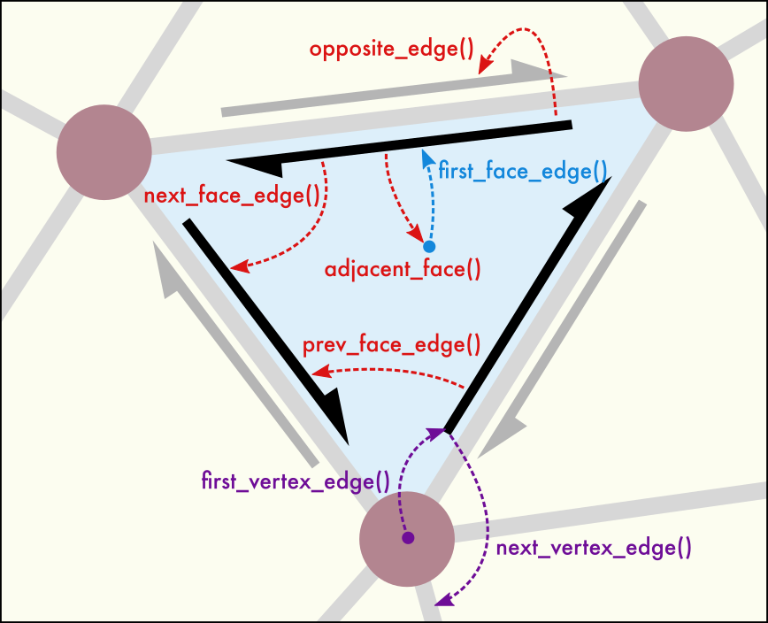
A halfedge is a directed edge \(a \to b\) connecting two vertices \(a\) and \(b\) – depicted as a half-arrow in the figure. A face is implicitly defined by a circular sequence of halfedges that bound the face. Typically, halfedges come in pairs. The halfedge \(a \to b\) and its opposite halfedge, \(b \to a\), form a pair that links two neighboring faces together. Thus, halfedge pairs are essential for forming a connected, two-dimensional surface manifold. The surface is said to be closed, i.e., it has no open boundaries if all halfedges of the mesh are associated with corresponding opposite halfedges (see
is_closed).For each vertex the topology object maintains a linked-list of directed halfedges leaving that vertex. It can be accessed through the
first_vertex_edge()andnext_vertex_edge()methods.For each face the topology object maintains a circular linked-list of directed halfedges bounding that face (in counter-clockwise winding order). It can be accessed through the
first_face_edge()andnext_face_edge()/prev_face_edge()methods.Tip
All query methods of this class are vectorized, which means they are able to process an array of arguments in a single function call and will return a corresponding array of results. The advantage of this is that the loop over the elements in the argument array runs entirely on the C++ side, which is typically much faster than a for-loop in Python. For example, to generate a list with the first halfedge of every mesh face:
# Version 1: vectorized function call (fast)
edges = mesh.topology.first_face_edge(range(mesh.topology.face_count))

# Version 2: explicit loop (slow)
edges = [mesh.topology.first_face_edge(face) for face in range(mesh.topology.face_count)]
- count_face_edges(face: int) int
Returns the number of halfedges that bound face. See the code example for
next_face_edge()to learn how this method works.
- count_manifolds(edge: int) int
Given a halfedge, this method returns the number of surface manifolds that meet at the edge. This is useful to identify triple junctions in a grain boundary network, for example. For halfedges that are located at the boundary of an open surface mesh, the method returns 1. For halfedges that are part of a regular two-sided manifold, the method returns 2.
See also
- count_vertex_edges(vertex: int) int
Returns the number of halfedges that leave vertex. See the code example for
next_vertex_edge()to learn how this method works.
- property edge_count: int
Total number of halfedges in the
SurfaceMesh. This property is read-only. Halfedges are created automatically bySurfaceMesh.create_face()orSurfaceMesh.create_faces()when adding new faces to the mesh topology.
- property face_count: int
Number of faces in the
SurfaceMesh. This is always equal to thecountof theSurfaceMesh.facesproperty container.This property is read-only. Use
SurfaceMesh.create_face()orSurfaceMesh.create_faces()to add new faces to the mesh.
- find_edge(face: int, vertex1: int, vertex2: int) int
Given a face, finds the halfedge of that face which leads from vertex1 to vertex2. If no such halfedge exists, returns -1.
This method can be used to quickly find the edge connecting two vertices of a face without the need to explicitly visit and check each edge bounding the face.
- first_edge_vertex(edge: int) int
Returns the vertex the given halfedge is leaving from. To retrieve the vertex the halfedge is leading to, call
second_edge_vertex().
- first_face_edge(face: int) int
Returns some halfedge bounding the given face. Given that first halfedge, all other halfedges bounding the same face can be visited using
next_face_edge()orprev_face_edge().
- first_face_vertex(face: int) int
Given a face, this method returns some vertex of that face. This is equivalent to retrieving the vertex to which the first halfedge of the face is connected to, i.e.
first_edge_vertex(first_face_edge(face)).
- first_vertex_edge(vertex: int) int
Returns the head halfedge from the linked list of halfedges leaving vertex. Subsequent halfedges from the linked list can be retrieved with
next_vertex_edge(). If no halfedges are connected to vertex, the method returns -1.
- has_opposite_edge(edge: int) bool
Returns whether the given halfedge edge is associated with a corresponding reverse halfedge bounding an adjacent face in the same manifold. This is equivalent to checking the return value of
opposite_edge(), which returns -1 to indicate that edge does not have an opposite edge.
- has_opposite_face(face: int) bool
Returns whether face is part of a two-sided manifold. A face that is part of a two-sided manifold has a ‘partner’ face with opposite orientation, which can be retrieved through the
opposite_face()method.
- property is_closed: bool
This is a read-only property indicating whether the surface mesh is fully closed. In a closed mesh, all faces are connected to exactly one adjacent face along each of their halfedges. That means the mesh presents a two-dimensional surface manifold without borders. Furthermore, a closed mesh divides space into an “interior” and an “exterior” region.
Added in version 3.7.9.
- next_face_edge(edge: int) int
Given the halfedge edge bounding some face, this method returns the following halfedge when going around the face in forward direction (counter-clockwise - when looking at the front side of the face). All halfedges of the face form a circular sequence - without a particular beginning or end. You can loop over this circular sequence in forward or backward direction with the
next_face_edge()andprev_face_edge()methods. Given some mesh face, you can obtain a first halfedge through thefirst_face_edge()method.The following code example shows how to visit all halfedges of a face in order. Since the halfedges form a circular linked list, we have to remember which edge we started from to terminate the loop once we reach the first edge again:
def count_edges(mesh: SurfaceMesh, face: int) -> int:
    start_edge = mesh.topology.first_face_edge(face)
    count = 1
    edge = mesh.topology.next_face_edge(start_edge)
    while edge != start_edge:
        assert mesh.topology.adjacent_face(edge) == face
        count += 1
        edge = mesh.topology.next_face_edge(edge)
    return count

# The function defined above is equivalent to SurfaceMeshTopology.count_face_edges():
assert count_edges(mesh, 0) == mesh.topology.count_face_edges(0)
- next_manifold_edge(edge: int) int
Advanced method to visit all surface manifolds meeting at an edge (e.g. along a triple junction in a grain boundary network). Given a halfedge, this method returns the halfedge that is part of the next manifold and which connects the same two mesh vertices.
The manifold information may only be available in certain types of surface meshes, such as those generated by the
ConstructSurfaceModifierwhen theidentify_regionsoption is turned on.See also
- next_vertex_edge(edge: int) int
Returns another halfedge leaving from the same vertex as edge. Together with
first_vertex_edge()this method allows you to iterate over all halfedges connected to some vertex. When the end of the vertex’ edge list has been reached, the method returns -1.The following example demonstrates how to visit all outgoing halfedges of some vertex and count them:
def count_edges(mesh: SurfaceMesh, vertex: int) -> int:
    count = 0
    edge = mesh.topology.first_vertex_edge(vertex)
    while edge != -1:
        assert mesh.topology.first_edge_vertex(edge) == vertex
        count += 1
        edge = mesh.topology.next_vertex_edge(edge)
    return count

# The function defined above is equivalent to SurfaceMeshTopology.count_vertex_edges():
assert count_edges(mesh, 0) == mesh.topology.count_vertex_edges(0)
- opposite_edge(edge: int) int
Given the halfedge edge, returns the reverse halfedge that bounds an adjacent face. This opposite halfedge connects the same two vertices as edge but in reverse order. You can use this method to determine whether the face bounded by edge has a neighboring face that is part of the same manifold:
def get_neighboring_face(mesh: SurfaceMesh, edge: int) -> int:
    opp_edge = mesh.topology.opposite_edge(edge)
    if opp_edge == -1: return -1
    assert mesh.topology.first_edge_vertex(edge) == mesh.topology.second_edge_vertex(opp_edge)
    assert mesh.topology.second_edge_vertex(edge) == mesh.topology.first_edge_vertex(opp_edge)
    return mesh.topology.adjacent_face(opp_edge)
You may call the convenience method
has_opposite_edge()to determine whether a halfedge is associated with a corresponding opposite halfedge. If the surface mesh does not form a closed manifold, the halfedges at the boundary of the manifold do not have opposite halfedges, because there are no adjacent faces where the surface terminates.
- opposite_face(face: int) int
Returns the face on the opposite side of the two-sided manifold, or -1 if the manifold is one-sided. The returned face shares the same vertices with face but in reverse order. Note that
opposite_face(opposite_face(face))==face.
- prev_face_edge(edge: int) int
Given the halfedge edge bounding some face, this method returns the previous halfedge going around that face in backward direction (clockwise - when looking at the front side of the face). All halfedges of a face form a circular sequence - without a particular beginning or end. You can loop over this circular sequence in forward or backward direction with the
next_face_edge()andprev_face_edge()methods.
- second_edge_vertex(edge: int) int
Returns the vertex the given halfedge is leading to. To retrieve the vertex the halfedge is leaving from, call
first_edge_vertex().
- property vertex_count: int
Number of vertices in the
SurfaceMesh. This is always equal to thecountof theSurfaceMesh.verticesproperty container.This property is read-only. Use
SurfaceMesh.create_vertices()to add new vertices to the mesh.
- class ovito.data.TriangleMesh
Base:
ovito.data.DataObjectThis data object type stores a three-dimensional mesh made of vertices and triangular faces. Such a mesh can describe general polyhedral geometry to be visualized side by side with the particle simulation data.
Typically, triangle meshes are imported from external geometry data files (e.g. STL, OBJ, VTK formats) using the
import_file()function. See also the corresponding section of the OVITO user manual. All triangle meshes in a data collection are accessible through theDataCollection.triangle_meshesdictionary view.Note that the
SurfaceMeshclass is a second object type that can represent surface geometries, just like aTriangleMesh. In contrast to triangle meshes, surface meshes may be embedded in periodic simulation domains and are closed manifolds in most cases. Furthermore, surface meshes can store arbitrary per-vertex and per-face property values – something triangle meshes cannot do. A triangle mesh is a more low-level data structure, which can be sent directly to a GPU for rendering. A surface mesh, in contrast, is a more high-level data structure, which gets automatically converted to a triangle mesh for visualization.The visual appearance of the triangle mesh is controlled through the attached
TriangleMeshViselement (seeDataObject.visfield of base class).A triangle mesh consists of \(n_{\mathrm{v}}\) vertices and \(n_{\mathrm{f}}\) triangular faces. These counts are exposed by the class as attributes
vertex_countandface_count. Each face connects three vertices of the mesh, and several faces may share a vertex. The faces are stored as triplets of zero-based indices into the vertex list.- property face_count: int
The number of triangular faces of the mesh, \(n_{\mathrm{f}}\).
- Default:
0
- get_faces() NDArray[int32]
Returns the list of triangles of the mesh as a NumPy array of shape \((n_{\mathrm{f}}, 3)\). The array contains for each face three zero-based indices into the mesh’s vertex list as returned by
get_vertices(). The returned face array holds a copy of the internal data managed by theTriangleMesh.
- get_vertices() NDArray[float64]
Returns the xyz coordinates of the vertices of the mesh as a NumPy array of shape \((n_{\mathrm{v}}, 3)\). The returned array holds a copy of the internal vertex data managed by the
TriangleMesh.
- set_faces(vertex_indices: ArrayLike)
Sets the faces of the mesh. vertex_indices must be an array-like object of shape \((n_{\mathrm{f}}, 3)\) containing one integer triplet per triangular face. Each integer is a zero-based index into the mesh’s vertex list. The
TriangleMeshcopies the data from the array into its internal storage. If necessary, the value offace_countis automatically adjusted to match the first dimension of the vertex_indices array.
- set_vertices(coordinates: ArrayLike)
Sets the xyz coordinates of the vertices of the mesh. coordinates must be an array-like object of shape \((n_{\mathrm{v}}, 3)\). The
TriangleMeshcopies the data from the array into its internal storage. If necessary, the value ofvertex_countis automatically adjusted to match the first dimension of the coordinates array.
- class ovito.data.Vectors
Base:
ovito.data.PropertyContainerThe
Vectorsclass represents a set of 3D arrow glyphs rendered by aVectorVisvisual element. You can add an instance of this class to aDataCollectionusing theDataCollection.vectors.create()method.You can retrieve existing
Vectorsobjects from a pipeline’s output data collection through theDataCollection.vectorsdictionary view. EachVectorsobject has a uniqueidentifiername that serves as a lookup key.Vectorsobjects are always associated withVectorViselement, which controls the visual appearance of the arrows in rendered images. You can access the visual element through thevisattribute provided by theDataObjectbase class. TheVectorViselement provides the capability to visualize a scalar quantity associated with each vector using pseudo-color mapping.The
Vectorscontainer uses the following standard properties with predefined names and data layouts. Additional per-arrow properties may be added using thecreate_property()method of the base class.Property name
Python access
Data type
Component names
Color
float32
R, G, B
Direction
float64
X, Y, Z
Position
float64
X, Y, Z
Selection
int8
Transparency
float32
Added in version 3.11.0.
- property colors: Property | None
The
Propertydata array for theColorstandard vector property; orNoneif that property is undefined. Usecreate_property()to add the property to the container if necessary. Usecolors_(with an underscore) to access an independent copy of the array, whose contents can be safely modified in place.
- property directions: Property | None
The
Propertyarray containing the XYZ components of the vectors (standard property Direction). May beNoneif the property is not defined yet. Usecreate_property()to add the property to the container if necessary. Usedirections_(with an underscore) to access an independent copy of the array, whose contents can be safely modified in place.
- property positions: Property | None
The
Propertyarray containing the XYZ coordinates of vectors’ base points (standard property Position). May beNoneif the property is not defined yet. Usecreate_property()to add the property to the container if necessary. Usepositions_(with an underscore) to access an independent copy of the array, whose contents can be safely modified in place.
- property selection: Property | None
The
Propertydata array for theSelectionstandard vectors property; orNoneif that property is undefined.
- property transparencies: Property | None
The
Propertyarray containing the transparency values (standard property Transparency) of the vectors. May beNoneif the property is not defined yet. Usecreate_property()to add the property to the container if necessary. Usetransparencies_(with an underscore) to access an independent copy of the array, whose contents can be safely modified in place.
- class ovito.data.VoxelGrid
Base:
ovito.data.PropertyContainer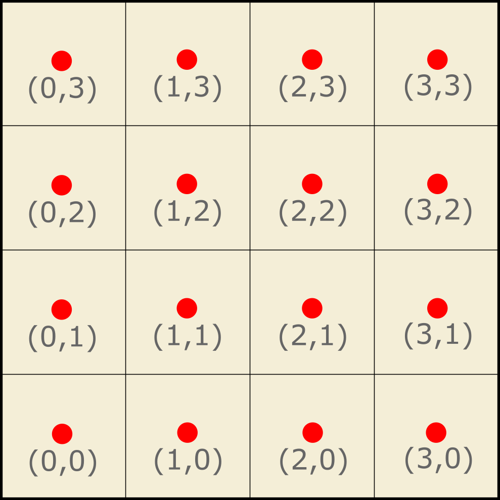
Cell-data grid
A two- or three-dimensional structured grid. Each cell (voxel) of the uniform grid is of the same size and shape. The overall geometry of the grid, its
domain, is specified by the attachedSimulationCellobject, which describes a three-dimensional parallelepiped or a two-dimensional parallelogram. See also the corresponding user manual page for more information on this object type.The
shapeproperty of the grid specifies the number of data points uniformly distributed along each cell vector of the domain. The size of individual voxels depends on the overall domain size as well as the number of data points in each spatial direction. See thegrid_typeproperty, which controls whether the data values of the uniform grid are associated with the voxel interiors or the vertices (grid line intersections).
Point-data grid
Each data point or voxel of the grid may be associated with one or more field values. The data of these voxel properties is stored in standard
Propertyarray objects, similar to particle or bond properties. Voxel properties can be accessed by name through the dictionary interface that theVoxelGridclass inherits from itsPropertyContainerbase class.Voxel grids can be loaded from input data files, e.g. a CHGCAR file containing the electron density computed by the VASP code, or they can be dynamically generated within OVITO. The
SpatialBinningModifierlets you project the information associated with the unstructured particle set to a structured voxel grid.Given a voxel grid, the
CreateIsosurfaceModifiercan then generate aSurfaceMeshrepresenting an isosurface for a field quantity defined on the voxel grid.Example
The following code example demonstrates how to create a new
VoxelGridfrom scratch and initialize it with data from a NumPy array:# Starting with an empty DataCollection: data = DataCollection() # Create a new SimulationCell object defining the outer spatial dimensions # of the grid and the boundary conditions, and add it to the DataCollection: cell = data.create_cell( matrix=[[10,0,0,0],[0,10,0,0],[0,0,10,0]], pbc=(True, True, True) ) # Generate a three-dimensional Numpy array containing the grid cell values. nx = 10; ny = 6; nz = 8 field_data = numpy.random.random((nx, ny, nz)) # Create the VoxelGrid object and give it a unique identifier by which it can be referred to later on. # Link the voxel grid to the SimulationCell object created above, which defines its spatial extensions. # Specify the shape of the grid, i.e. the number of cells in each spatial direction. # Finally, assign a VoxelGridVis visual element to the data object to make the grid visible in the scene. grid = data.grids.create( identifier="field", domain=cell, shape=(nx,ny,nz), grid_type=VoxelGrid.GridType.CellData, vis_params={ "enabled": True, "transparency": 0.6 } ) # Add a new property to the voxel grid cells and initialize it with the data from the NumPy array. # Note that the data must be provided as linear (1-dim.) array with the following type of memory layout: # The first grid dimension (x) is the fasted changing index while the third grid dimension (z) is the # slowest varying index. In this example, this corresponds to the "Fortran" memory layout of Numpy. grid.create_property('Field Value', data=field_data.flatten(order='F')) # Instead of the flatten() method above, we could also make use of the method VoxelGrid.view() # to obtain a 3-dimensional view of the property array, which supports direct assignment of grid values. field_prop = grid.create_property('Field Value', dtype=field_data.dtype, components=1) grid.view(field_prop)[...] = field_data # For demonstration purposes, compute an isosurface on the basis of the VoxelGrid created above. data.apply(CreateIsosurfaceModifier(operate_on='voxels:field', property='Field Value', isolevel=0.7))
The
VoxelGridcontainer uses the following standard properties with predefined names and data layouts. Additional per-voxel properties may be added using thecreate_property()method of the base class.Property name
Python access
Data type
Component names
Color
float32
R, G, B
- property domain: SimulationCell | None
The
SimulationCelldescribing the (possibly periodic) domain which this grid is embedded in. Note that this cell generally is independent of and may be different from thecellfound in theDataCollection.- Default:
None
- property grid_type: VoxelGrid.GridType
This attribute specifies whether the values stored by the grid object are associated with the voxel cell centers or the grid points (vertices). Possible values are:
VoxelGrid.GridType.CellData(default)VoxelGrid.GridType.PointData
A
CellDatagrid represents a field where the sampling points are located in the centers of the voxel cells. This grid type is typically used for volumetric datasets, which represent some quantity within the discrete voxel cell volumes.
A
PointDatagrid represents a field where the sampling points are located at the intersections of the grid lines. Note that, for this grid type only, the type of boundary conditions of the grid’sdomainaffect the uniform spacing of the sampling points:
4 x 4 point-data grid (left: non-periodic domain, right: periodic domain)
- Default:
VoxelGrid.GridType.CellData
- property shape: tuple[int, int, int]
A 3-tuple specifying the number of sampling points along each of the three cell vectors of the
domain.For two-dimensional grids, for which the
is2Dproperty of thedomainis set, the third entry in thisshapetuple must be equal to 1.Assigning a new shape to the grid automatically resizes the one-dimensional data arrays stored by this
PropertyContainerand updates itsPropertyContainer.countproperty to match the product of the three dimensions, i.e. the total number of data points.- Default:
(0, 0, 0)
- view(key)
Returns a shaped view of the given grid property, which reflects the 2- or 3-dimensional
shapeof the grid.- Parameters:
key (str | Property) – The name of the grid property to look up. May include the underscore suffix to make the property mutable. Alternatively, you can directly specify a
Propertyobject from thisVoxelGrid.- Returns:
A NumPy view of the underlying property array.
- Return type:
Because the
VoxelGridclass internally uses linearPropertyarrays to store the voxel cell values, you normally would have to convert back and forth between the linear index space of the underlying property storage and the 2- or 3-dimensional grid space to access individual voxel cells.The
view()helper method frees you from having to map grid coordinates to array indices because it gives you a shaped NumPy view of the underlying linear storage, which reflects the correct multi-dimensional shape of the grid. For 3-dimensional grids, the ordering of the view’s dimensions is \(x,y,z[,k]\), with \(k\) being an extra dimension that is only present if the accessed property is a vector field quantity. For 2-dimensional grids, the ordering of the view’s dimensions is \(x,y[,k]\).The returned view lets you conveniently access the values of individual grid cells based on multi-dimensional grid coordinates. Here, as an example, the scalar field property
c_aveof a 3-dimensional voxel grid:nx, ny, nz = grid.shape field = grid.view('c_ave') for x in range(nx): for y in range(ny): for z in range(nz): print(field[x,y,z])
Added in version 3.9.0.