Spatial binning pro

The Spatial Binning modifier generates a 1-, 2-, or 3-dimensional grid covering the entire simulation domain, subdividing the cell into uniformly shaped bins. These bins are aligned with the edges of the simulation cell — even if the cell is sheared — ensuring consistent spatial resolution across the domain.
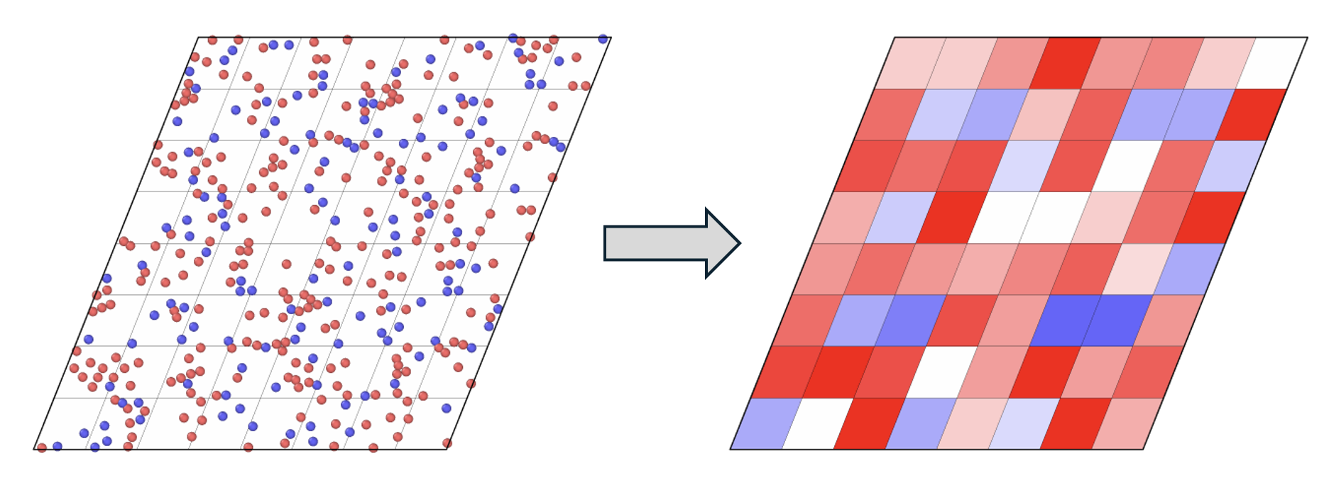
This modifier can be used to compute a coarse-grained field representation from discrete particles or dislocation lines.
Particles are assigned to the appropriate bins based on their positions. Within each bin, a specified reduction operation is performed on a selected particle property, which may be scalar or vector-valued. This process projects particle-based data onto a structured grid, producing a coarse-grained field representation.
You can choose between different reduction operations, e.g., sum, average (mean), minimum or maximum, to be applied per grid cell.
- Dislocations
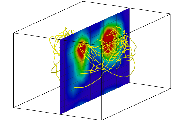
For dislocation lines, the modifier calculates the scalar dislocation density and the Nye tensor within each grid cell. The local dislocation density is expressed in units of 1/length2. When projecting to a 1- or 2-dimensional binning grid, the dislocation density and Nye tensor are still calculated from the 3-dimensional cell volume.
Note: This mode is only supported for orthogonal, axis-aligned simulation cells.
The calculation method follows the approach described in section 2 of:
A preprint is available here.
Added in version 3.11.0.
Data output options
For 1D binning, the computed data is accessible via the data inspector and can be exported as a text file.
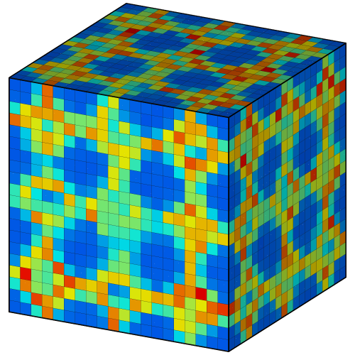
For 3D binning, the output is stored as a voxel grid, which can be visualized using 3D volume rendering or the Create isosurface and Slice modifiers.
2D and 3D grid data can also be exported using OVITO’s file export function. Use the VTK Voxel Grid output format.
Parameters
- Operate on
Selects whether to bin data from particles or dislocation lines.
- Input property (only for particles)
The particle property to apply the reduction operation to. Select <None> to use a uniform value of 1 for all particles, which enables counting particles (sum) or computing the number density (sum divided by bin volume) in each grid cell.
- Use only selected elements (only for particles)
Restricts the computation to the currently selected subset of particles.
- Binning direction(s)
Specifies which cell axes to use for binning, determining also the grid’s dimensionality.
- Number of bins
Number of bins along each of the active binning directions.
- Reduction operation (only for particles)
- Determines how data is aggregated per bin. Options include:
sum
mean
min
max
sum divided by bin volume (useful for computing densities or pressure from per-atom quantities like virial)
- Compute first derivative
Calculates the first derivative of the binned data using a finite-difference approximation. Only available for 1D binning. Useful, for example, in computing local shear rate from a velocity profile.
- Fix property axis range
If enabled, the display range for the binned property (or color scale for 2D grids) will be fixed to the values entered in the From and To fields. Otherwise, the range is auto-scaled based on data values.
Usage example: Counting particle types to compute local stoichiometry
This example demonstrates how to use the Spatial Binning modifier to compute the local concentration of each particle species (stoichiometry).
Each particle’s chemical identity is stored in the Particle Type property as an integer type ID. For a ternary alloy, let’s assume the following mapping:
1 (Ni)
2 (Co)
3 (Cr)
Since Particle Type is a categorical property, computing a simple reduction such as mean is not meaningful.
Instead, we want to count how many particles of each type fall into each spatial bin.
To achieve this, we first need to expand the Particle Type property into a vectorial property, let’s call it Type Count,
where each component of the vector corresponds to a different particle type. A single particle will have a value of 1 in the component corresponding
to its type, and 0 in all other components. The Compute property modifier can be used to create this new property:
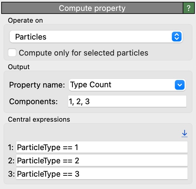
Enter “1, 2, 3” into the Components field to create a vector property with three components. Each expression
ParticleType == <type_id> will evaluate to 1 for particles of the corresponding type and 0 otherwise.
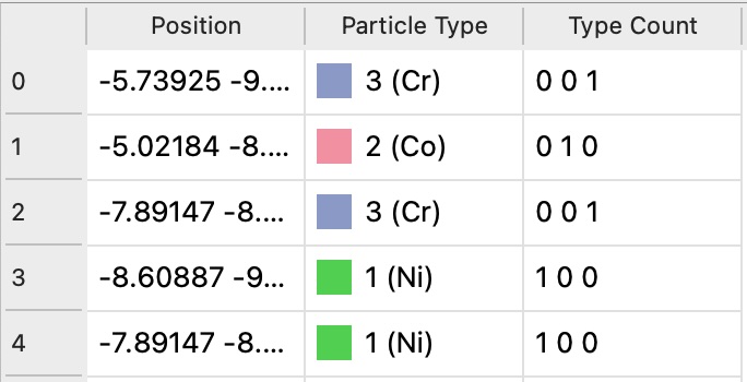
The data inspector panel shows the new Type Count property as a vectorial property with three components:
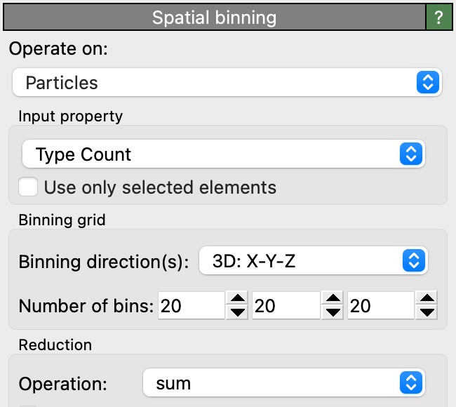
Now it is possible to use the Spatial Binning modifier to compute the number of particles of each type in each bin.
We select the Type Count property as input property and choose the sum reduction operation:
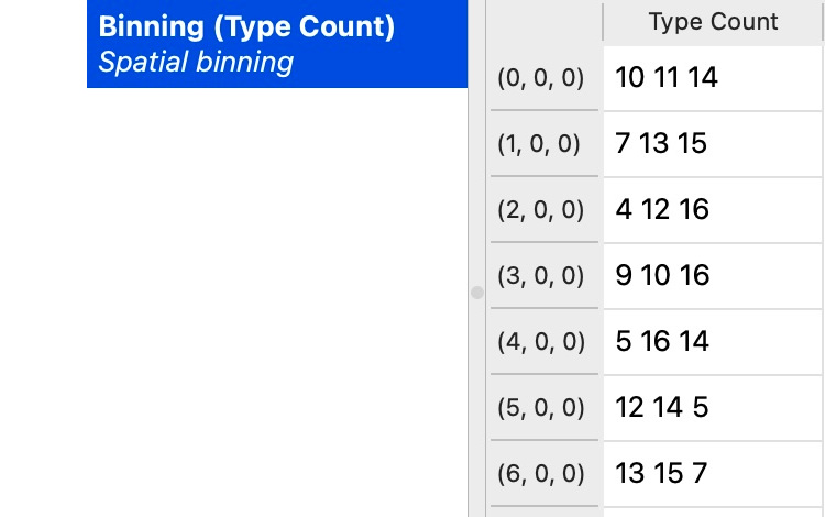
You can now compute derived quantities, such as local species concentrations, by applying another Compute property modifier to the resulting voxel grid.
See also
ovito.modifiers.SpatialBinningModifier (Python API)