Example FR2: Optimizing the performance of Example FR1

This example is based on Example FR1: Custom file reader loading particle properties and the simulation cell, before continuing please make sure that you are familiar with the code in that example.

In this example we will address the two performance critical issues found in that file reader:

1. For long trajectories, seeking to a requested frame by reading all lines preceding that frame will become slower and slower for later frames.

2. For simulations containing many atoms, performing many property assignments such as type_property[i] = ... can become a bottleneck.

Seeking to the requested frame

As a first optimization we save the byte offset to the start of each frame instead of the line number. This allows the file reader to jump directly to the correct position inside the file instead of sequentially stepping through it line by line until the requested frame is found.

This requires two changes. First, the scan method needs to store byte offsets instead of line numbers. The current byte offset of the file pointer can be obtained with the tell() method, which is not available within a for line in f: loop. Therefore, the for loop gets replaced by a while loop calling readline() explicitly:

def scan(self, filename: str, register_frame: Callable[..., None]):
    with open(filename, "r") as f:
        while line := f.readline():
            if line.startswith("Timestep "):
                # Byte offset of the beginning of the current line:
                offset = f.tell() - len(line.encode("utf-8"))
                register_frame(frame_info=offset, label=line.strip())
            yield

Since the tell() method is not particularly fast, it is called only after a line starting a new frame has been identified. The byte offset reported by tell() must be shifted by the length of the current line in bytes, because reading the line has already advanced the file pointer. The yield statement gives OVITO Pro the chance to update its user interface and to interrupt the scan if needed (see Long-running computations).

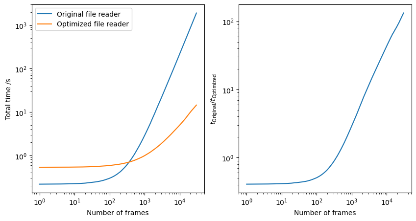
Quick benchmarks show that the new scan method is about 1.5 to 2 times slower than the old one. However, the speedup of the parse method more than makes up for this difference: instead of reading all lines preceding the requested frame, the parse method can now jump directly to the beginning of the frame using a single seek call (see the complete code below).

To benchmark these code changes we measured the total time to step through a trajectory file containing 30,000 frames of ~20 atoms per frame. Here we can see that the optimized version of the file reader takes about 14 seconds to open all 30,000 frames, while the old, unoptimized version, takes about 32 minutes.

Minimizing OVITO / Python data exchange

In a next step we want to optimize the assignment of particle properties. Recall that the old version of the file reader developed in Example FR1: Custom file reader loading particle properties and the simulation cell copies both the positions and particle types for each particle individually from Python into OVITO memory. This takes time and can be optimized by collecting all data in Python / numpy and copying it into OVITO in one go.

This approach allows for an optimization of the conversion between reduced and Cartesian coordinates. While the original implementation transformed the coordinates for each particle individually, the usage of numpy.einsum now allows for vectorization and therefore acceleration of this calculation.

Be aware, that this optimization increases the memory requirements of the file reader.

This leads to the following updated parse method:

def parse(self, data: DataCollection, filename: str, frame_info: int, **kwargs: Any):
    with open(filename, "r") as f:
        # Jump directly to the beginning of the requested trajectory frame
        f.seek(frame_info)

        data.attributes["Timestep"] = int(f.readline().split()[1])

        cell = data.create_cell([[0, 0, 0, 0], [0, 0, 0, 0], [0, 0, 0, 0]], pbc=(True, True, True))
        for i in range(3):
            cell[:, i] = [float(c) for c in f.readline().split()]

        particle_count = int(f.readline().split()[1])
        particles = data.create_particles(count=particle_count)
        type_property = particles.create_property("Particle Type")
        position_property = particles.create_property("Position")
        f.readline()

        # Collect the particle data in NumPy arrays first:
        types = numpy.empty(particle_count, dtype=numpy.int32)
        positions = numpy.empty((particle_count, 4))
        positions[:, 3] = 1.0
        for i in range(particle_count):
            tokens = f.readline().split()
            types[i] = type_property.add_type_name(tokens[0], particles).id
            positions[i, :3] = [float(c) for c in tokens[1:4]]
            yield i / particle_count

        # Copy the data into the OVITO properties in one go, converting all coordinates at once:
        type_property[...] = types
        position_property[...] = numpy.einsum("ij,kj->ki", cell, positions)

First, the method pre-allocates NumPy arrays for the particle types and positions. The position array has four components per particle, because the conversion from reduced to Cartesian coordinates is the multiplication of the 3x4 cell matrix \(M\) with the vector \(p = (x_\mathrm{r}, y_\mathrm{r}, z_\mathrm{r}, 1)\).

The loop over all particles then stores the data read from the file in the NumPy arrays instead of the particle properties, keeping the coordinates in reduced form. Finally, the method copies the type array into the Particle Type property in one go and uses numpy.einsum to convert all particle coordinates from reduced to Cartesian coordinates with a single, vectorized matrix multiplication.

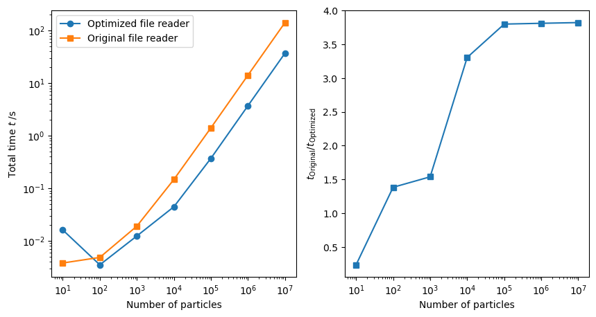
To benchmark these code changes we measured the total time to load a single frames containing 10 to 10,000,000 atoms. Here we can see that the optimized version of the file reader takes about 37 seconds to open the largest file, while the old, unoptimized version, takes about 142 seconds.

Final thoughts

In this example we showed two common optimizations that can be implemented for a custom file reader. We saw that optimizing the seek behavior is really important for long trajectories, while the optimized data transfer becomes most relevant for trajectories containing a large number of atoms. Each project comes with its own challenges and only repeated measurements and optimizations can help you to build a fast and reliable file reader.