Data model
This chapter describes how OVITO represents the data that flows through a pipeline: particles, bonds, the simulation cell, and everything else that gets loaded from a simulation file or computed by modifiers. The next chapter, Manipulating data, then discusses how to modify this data.
Data collections and data objects
OVITO organizes a dataset into data objects, each representing one part of the dataset. For example, a
SimulationCell object stores the simulation box geometry and the periodic boundary conditions, and a
Particles object stores the particles and their properties. For each type of data object, there is a
corresponding Python class in the ovito.data module, all deriving from the common base class DataObject.
Data objects can contain other data objects. The Particles object, for example, manages a set of
Property objects, each storing the values of one particle property, and it may contain a
Bonds object, which in turn manages the properties of the bonds:
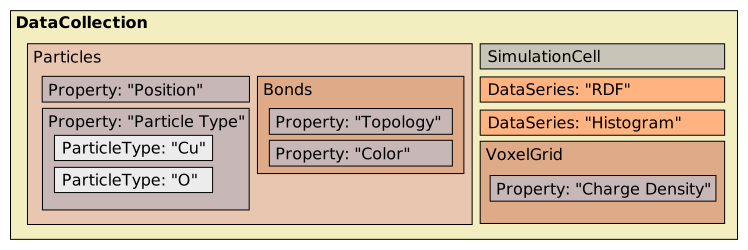
A DataCollection is the top-level container holding all data objects of one dataset.
It is what Pipeline.compute() returns, and it is what a modifier receives as input and modifies.
The DataCollection class provides fields for accessing the different kinds of data objects it may contain:
Field |
Contents |
|---|---|
The |
|
The |
|
A dictionary of global attributes, i.e. scalar values associated with the dataset as a whole |
|
A dictionary of data tables, e.g. histograms or other results computed by modifiers |
|
A dictionary of |
|
A dictionary of |
|
A dictionary of |
|
A dictionary of |
|
The |
|
The |
|
A dictionary of |
Fields that refer to a dictionary let you look up data objects by their identifier, because a dataset
may contain several objects of the same kind. The objects field gives you the flat list of all top-level data objects.
Important
A DataCollection represents a single frame of a simulation trajectory. Pipelines operate on one
frame at a time, and a trajectory is represented by a sequence of DataCollection objects, one for each frame.
In the following sections, we’ll use the data returned by this pipeline as an example:
from ovito.io import import_file
from ovito.modifiers import CommonNeighborAnalysisModifier

pipeline = import_file("input/simulation.dump")
pipeline.modifiers.append(CommonNeighborAnalysisModifier())
data = pipeline.compute()
Particles
OVITO uses a property-based representation of particles. Rather than storing a list of particle objects, the Particles
container stores a set of arrays, one for each particle property such as position, type, mass, or color. Each array holds the values
for all N particles in the system. A particle is thus nothing more than an index into these arrays.
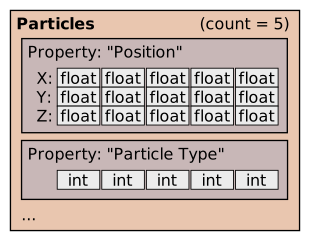
The Particles container behaves like a Python dictionary mapping property names to Property arrays.
Its count attribute reports the number of particles:
print(data.particles.count)
print(list(data.particles.keys()))
7071
['Position', 'Particle Identifier', 'peatom', 'Particle Type', 'Force', 'Structure Type', 'Color']
OVITO defines a set of standard particle properties such as Position, Particle Type, or Color,
which have a specific meaning to the program and a prescribed data layout. Only Position is mandatory; all other properties are optional.
Properties with other names, like peatom in this example, are user-defined properties. OVITO treats them as generic numeric data.
Note
Many file readers map the columns of the input file to standard properties automatically.
The import_file() function lets you control this mapping if necessary (see File I/O).
Multiple particle systems
A data collection can contain more than one particle system. DataCollection.particles
always refers to the main particle system. Secondary particle systems, generated for example by the
ClusterAnalysisModifier, are accessible through the
DataCollection.particle_systems dictionary:
from ovito.modifiers import ClusterAnalysisModifier

cluster_pipeline = import_file("input/simulation.dump")
cluster_pipeline.modifiers.append(ClusterAnalysisModifier(cutoff=2.8, sort_by_size=True))
cluster_data = cluster_pipeline.compute()

print(list(cluster_data.particle_systems.keys()))
clusters = cluster_data.particle_systems['clusters']
print(clusters.count)              # Number of clusters
print(clusters.positions[0])       # Center of mass of the largest cluster
Each secondary particle system is a Particles container in its own right. In the case of the cluster list,
each “particle” represents one cluster, located at the cluster’s center of mass.
Property arrays
A Property object is an array with one element per particle. You can look it up by name or, for standard properties,
through a convenience field of the Particles container:
positions = data.particles["Position"]     # Look up a property by name
positions = data.particles.positions       # Same, using the convenience field
print(positions[0])                        # xyz coordinates of the first particle
print(positions.shape, positions.dtype)
[-65.8951646  37.7911415 -18.5904408]
(7071, 3) float64
A property can be scalar, i.e. a one-dimensional array of shape (N,), or vectorial, i.e. a two-dimensional array of shape (N, M) with M
components, like the three components of the Position property. Property objects behave like NumPy arrays and can
be passed to any NumPy function:
import numpy

energies = data.particles["peatom"]
print("Mean energy:", numpy.mean(energies))
print("Index of particle with lowest energy:", numpy.argmin(energies))
print("Particles above z=0:", numpy.count_nonzero(positions[:,2] > 0.0))
Tip
Use vectorized NumPy operations on entire property arrays whenever possible. Looping over particles in Python code is typically much slower.
Property arrays obtained from a DataCollection are read-only. The next chapter
explains how to modify them.
All values of a property share the same data type, which is reported by its dtype attribute:
64-bit floating-point numbers for continuous quantities such as positions, 32-bit integers for typed properties such as Particle Type,
64-bit integers for unique identifiers such as Particle Identifier, and 8-bit integers for flags such as Selection.
Standard properties with real values can optionally be stored in single precision (float32) to reduce memory usage, see Floating-point precision of standard properties.
User-defined properties may also store text strings. See Data types for the complete list of supported data types.
Typed properties
Some integer properties, most importantly Particle Type, encode a discrete type for each particle as a numeric ID. The property carries a
list of ElementType objects defining the types, which you can access through its types attribute.
Each type has a unique numeric id, an optional name, and further attributes
controlling the visualization, e.g. the display color and radius of particles of that type:
protein = import_file("input/1AKI.gro").compute()
type_property = protein.particles.particle_types
print(type_property[:8])                   # Numeric type IDs of the first 8 atoms
for t in type_property.types:
    print(t.id, t.name, t.color, t.radius)
[7 1 1 1 6 1 6 1]
1 H [1. 1. 1.] 0.46000000834465027
6 C [0.56470591 0.56470591 0.56470591] 0.7699999809265137
7 N [0.1882353  0.3137255  0.97254902] 0.7400000095367432
8 O [1.         0.05098039 0.05098039] 0.7400000095367432
16 S [0.7 0.7 0. ] 1.0499999523162842
Note that type IDs are not necessarily consecutive. Use the type_by_name() method to look up the numeric ID of
a named type:
oxygen_type_id = type_property.type_by_name("O").id
print("Number of oxygen atoms:", numpy.count_nonzero(type_property == oxygen_type_id))
Some analysis modifiers produce typed properties, too. The CommonNeighborAnalysisModifier, for example, outputs
the Structure Type property, which classifies each particle as fcc, hcp, bcc, etc.:
structure_types = data.particles.structure_types
for t in structure_types.types:
    print(t.id, t.name, numpy.count_nonzero(structure_types == t.id))
0 Other 2746
1 FCC 4310
2 HCP 7
3 BCC 8
4 ICO 0
See Typed properties for more information.
Other property containers
The Particles class is a specialization of the generic PropertyContainer base class.
Several other kinds of data in OVITO are organized the same way – as a set of uniform elements with an arbitrary number of properties:
Bonds: the bonds between particles (see below)DataTable: tabulated data, where each column is a property (see below)VoxelGrid: structured grids, where the properties are associated with the grid cellsThe vertices, faces, and regions of a
SurfaceMeshCartoon: the residues of a protein backbone forming a cartoon representation
Everything described in this chapter for particle properties applies to these containers as well.
Bonds
Bonds between particles get loaded from the input file, if available, or created by modifiers such as the CreateBondsModifier.
They are stored in a Bonds container, which is part of the Particles object.
Like particles, bonds can have an arbitrary set of properties. The standard property Topology stores, for each bond, the indices of the two particles it connects:
molecule = import_file("input/nylon.data").compute()
bonds = molecule.particles.bonds
print("Number of bonds:", bonds.count)
print(list(bonds.keys()))
print(bonds.topology[:3])                  # Indices of the two atoms connected by each bond
Number of bonds: 42
['Topology', 'Bond Type', 'Periodic Image']
[[0 4]
 [0 3]
 [0 6]]
The bond topology array can be used to index particle property arrays. The following code calculates the length of each bond,
taking into account periodic boundary conditions with the help of the SimulationCell.delta_vector() method:
positions = molecule.particles.positions
topology = bonds.topology
bond_vectors = molecule.cell.delta_vector(positions[topology[:,0]], positions[topology[:,1]])
bond_lengths = numpy.linalg.norm(bond_vectors, axis=1)
print("Mean bond length:", numpy.mean(bond_lengths))
Element references
The Topology property of bonds is an example of an element reference: an integer property whose values are indices into
another property container. OVITO keeps track of such references explicitly. A reference property knows which container it refers to:
print(bonds.topology.reference_target) # The container the atom indices refer to
particles
When elements are deleted from or reordered in the referenced container, OVITO updates the references automatically. Bonds whose atoms get deleted are deleted along with them:
molecule = import_file("input/nylon.data").compute()
print("Before:", molecule.particles.count, "atoms,", molecule.particles.bonds.count, "bonds")

# Delete the first three atoms:
molecule.particles_.delete_indices([0, 1, 2])
print("After: ", molecule.particles.count, "atoms,", molecule.particles.bonds.count, "bonds")
Before: 44 atoms, 42 bonds
After:  41 atoms, 34 bonds
Some analysis modifiers output element references, too. For example, the ClusterAnalysisModifier assigns each particle to a cluster.
Its output particle property Cluster refers to the elements of the secondary clusters particle system,
which stores the size and other properties of each cluster.
A reference property can be used directly as an index array to look up information about the referenced elements:
cluster = data.particles["Cluster"]
print(cluster.reference_target)             # The particle property refers to the elements of this container
clusters = data.get(cluster.reference_target)
print(list(clusters.keys()))

# Look up the size of the cluster each particle belongs to:
particle_cluster_sizes = clusters["Cluster Size"][cluster]
You can declare your own reference properties using the reference parameter of the create_property() method:
from ovito.data import NearestNeighborFinder

# Determine the nearest neighbor of each atom and store its index as a new particle property:
finder = NearestNeighborFinder(1, molecule)
neighbor_indices, _ = finder.find_all()
molecule.particles_.create_property("Nearest Neighbor", data=neighbor_indices[:,0], reference=molecule.particles)
See Element references for more information, including how references appear in the expressions of modifiers such as the
ExpressionSelectionModifier.
Simulation cell
The SimulationCell object stores the three vectors spanning the simulation box and the position of its origin,
which together form a 3x4 matrix, plus the periodic boundary condition flags:
print(data.cell[...])       # 3x4 matrix: three cell vectors and the cell origin
print(data.cell.pbc)        # periodic boundary conditions
[[169.4019928   0.          0.        -84.7009964]
 [  0.        123.2969972   0.        -61.6484986]
 [  0.          0.         80.1464004 -40.0732002]]
(True, True, True)
The SimulationCell class provides several helper methods, e.g. for converting between Cartesian and reduced coordinates
or for computing distance vectors with the minimum image convention.
Global attributes
Global attributes are scalar values – numbers or strings – associated with a dataset as a whole. They are stored in the
DataCollection.attributes dictionary. File readers generate some attributes,
e.g. the simulation timestep number of the current frame or the name of the input file. Many modifiers output their results as global attributes,
e.g. the number of atoms classified as fcc by the CommonNeighborAnalysisModifier:
for name, value in data.attributes.items():
    print(f"{name:>32} = {value}")
                     SourceFrame = 0
                      SourceFile = /home/user/input/simulation.dump
                        Timestep = 0
CommonNeighborAnalysis.counts.OTHER = 2746
CommonNeighborAnalysis.counts.FCC = 4310
CommonNeighborAnalysis.counts.HCP = 7
CommonNeighborAnalysis.counts.BCC = 8
CommonNeighborAnalysis.counts.ICO = 0
The documentation of each modifier lists the attributes it outputs. In the graphical user interface, you can inspect the attributes of a
pipeline’s output in the data inspector. Global attributes can be exported to a text file
for all frames of a trajectory, see Writing output files, or displayed in rendered images using a TextLabelOverlay.
Data tables
Modifiers that compute tabulated results, e.g. histograms or radial distribution functions, output them as DataTable objects.
A data table is a specialized PropertyContainer, in which each column is a Property.
The DataCollection.tables dictionary lets you look up tables by their identifier:
print(data.tables.keys())
table = data.tables["structures"]
print(table.xy())
KeysView({'structures': DataTable()})
[[   0 2746]
 [   1 4310]
 [   2    7]
 [   3    8]
 [   4    0]]
The xy() method returns the table’s x and y columns as a single NumPy array, which is convenient for plotting.
In the graphical user interface, data tables are displayed as charts in the data inspector.
To write a data table to a text file, use the export_file() function with the txt/table format.
Surfaces, grids, and more
Besides particles, OVITO can represent various other kinds of data. Each has its own class in the ovito.data module,
whose documentation describes the data structure in detail:
SurfaceMesh: closed, triangulated surfaces embedded in a periodic domain, e.g. constructed by theConstructSurfaceModifieror theCreateIsosurfaceModifier. See also the user manual.VoxelGrid: two- or three-dimensional structured grids, e.g. charge density data loaded from a fileDislocationNetwork: dislocation lines extracted by theDislocationAnalysisModifierLines: polylines, e.g. particle trajectory lines generated by theGenerateTrajectoryLinesModifierVectors: arrow glyphs placed at arbitrary positionsTriangleMesh: general triangle meshes, e.g. loaded from an OBJ, STL, or VTK file
See also
Manipulating data – How to modify the data in a
DataCollectionVisual elements – How OVITO visualizes the different kinds of data objects