Rendering & visualization

Python scripts

This chapter explains how to render images and movies of the output of pipelines, and how to control the visual appearance of the data. The following example sets up a pipeline that colors the particles according to their potential energy. Remember that only pipelines that were added to the scene appear in rendered images:

from ovito.io import import_file
from ovito.modifiers import ColorCodingModifier

pipeline = import_file("input/simulation.dump")
pipeline.modifiers.append(ColorCodingModifier(property="peatom", gradient=ColorCodingModifier.Viridis()))
pipeline.add_to_scene()

Visual elements

OVITO separates the data from its visual representation. A data object, e.g. a SimulationCell, stores the information itself. A visual element attached to the data object, e.g. a SimulationCellVis, is responsible for turning this information into graphics in the viewports and rendered images. Visual elements have parameters controlling the appearance, e.g. the line width and color of the simulation box. They correspond to the visual elements listed in the pipeline editor of the desktop application.

You access the visual element of a data object through its vis attribute:

data = pipeline.compute()
data.particles.vis.radius = 0.9               # Default display radius of particles
data.cell.vis.line_width = 0.3                # Line width of the simulation box
data.cell.vis.rendering_color = (0.5, 0.5, 0.5)

Note

Unlike the data in a pipeline output snapshot, visual elements are not copied. The visual elements you access through the data returned by compute() are the same objects the pipeline uses to render its output. Changing their parameters therefore affects all subsequently rendered images.

All visual elements derive from the DataVis base class, whose enabled attribute turns the visualization of the data object on or off. For example, data.cell.vis.enabled = False hides the simulation box. The ovito.vis module documents all visual element types and their parameters.

Modifiers that output data meant to be visualized, e.g. the displacement vectors computed by the CalculateDisplacementsModifier, attach a visual element to the data they create. Such modifiers typically also give you direct access to the visual element through their vis attribute, e.g. CalculateDisplacementsModifier.vis.

Particle types

The display color and radius of particles are, by default, determined by their particle types. Since types are part of the data, not visual elements, you change them by inserting an EditTypesModifier into the pipeline:

from ovito.modifiers import EditTypesModifier

edit_types = EditTypesModifier()
pipeline.modifiers.insert(0, edit_types)
edit_types.edit_type(1, name="Cu", radius=1.3)
edit_types.edit_type(2, name="Zr", radius=1.6)

Viewports

A Viewport defines the virtual camera looking at the scene:

from ovito.vis import Viewport

viewport = Viewport(type=Viewport.Type.Perspective)
viewport.camera_dir = (-1, -1.5, -0.8)
viewport.fov = 0.6                            # Vertical field of view in radians
viewport.zoom_all()

Like the viewport windows of the desktop application, a Viewport can be of type Top, Front, Left, etc., or of type Perspective or Ortho, which let you orient the camera freely in space. Set the viewport type first, before setting any other camera parameters, because changing the type resets the camera orientation.

The camera_dir and camera_pos attributes control the viewing direction and position of the camera. For perspective views, fov specifies the vertical field of view angle; for parallel projections, it specifies the vertical size of the visible area in length units. The zoom_all() method positions the camera such that all objects in the scene are fully visible.

Tip

Setting up a good camera perspective by trial and error can be tedious. Instead, adjust the view interactively in OVITO Pro and use the Python code generator to obtain the corresponding camera parameters.

Rendering images

The Viewport.render_image() method renders an image of the scene as seen through the viewport:

viewport.render_image(filename="output/picture.png", size=(800, 600))

Besides writing the image to a file, the method returns it as a Qt QImage object, which you can process further in Python. Optional arguments control, for example, the background color, a transparent background (alpha=True), and the animation frame to render.

Overlays

Viewport layers add two-dimensional graphics on top of the rendered scene, e.g. a color legend or a text label showing the value of a global attribute. You attach them to a viewport’s overlays list:

from ovito.vis import ColorLegendOverlay, TextLabelOverlay
from ovito.qt_compat import QtCore

viewport.overlays.append(ColorLegendOverlay(
    modifier=pipeline.modifiers[-1],
    caption="Potential energy (eV)",
    orientation=QtCore.Qt.Orientation.Vertical,
    format_string="%.2f",
    alignment=QtCore.Qt.AlignmentFlag.AlignRight | QtCore.Qt.AlignmentFlag.AlignVCenter))
viewport.overlays.append(TextLabelOverlay(
    text="Timestep [Timestep]",
    pipeline=pipeline,
    alignment=QtCore.Qt.AlignmentFlag.AlignLeft | QtCore.Qt.AlignmentFlag.AlignTop,
    font_size=0.05))

The text of the TextLabelOverlay can contain references to global attributes in square brackets, which get replaced with their current values. Further layer types are the CoordinateTripodOverlay and the PythonViewportOverlay, which lets you draw arbitrary graphics with your own Python code (see User-defined viewport layers).

Outlines

The outlines_enabled option of render_image() draws outlines along the silhouettes of objects, which can improve the visual separation of objects in the picture:

viewport.render_image(filename="output/picture_outlines.png", size=(800, 600),
                      outlines_enabled=True, outlines_min_width=1.5)

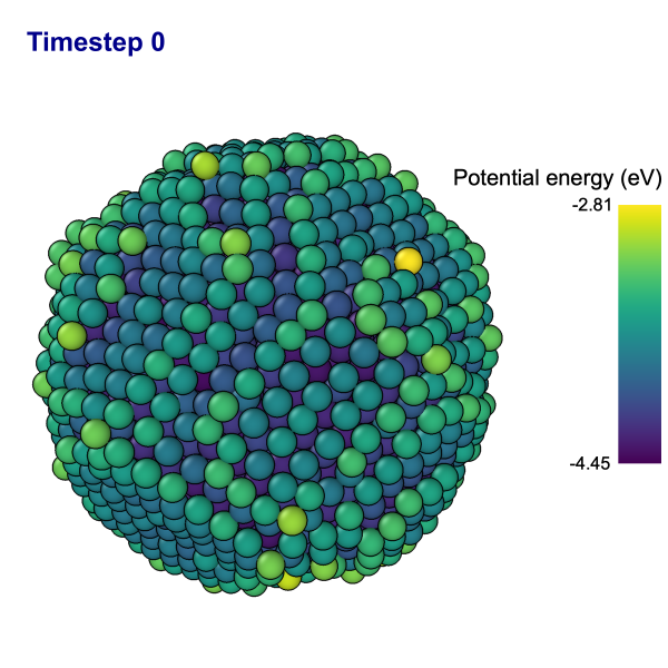
Rendered image showing particles colored by potential energy, with outlines, a color legend, and a text label.

The image on the right shows the result, including the viewport layers added above. Further parameters let you control the width and color of the outlines.

Rendering engines

OVITO provides several rendering engines, which differ in speed and visual quality:

StandardRenderer: Fast, GPU-accelerated rasterization (the default).
TachyonRenderer: Software-based ray tracing with ambient occlusion and shadows.
OSPRayRenderer: Software-based ray tracing with high visual fidelity, supporting semi-transparent objects and depth-of-field effects.
VisRTXRenderer: Hardware-accelerated ray tracing with global illumination on NVIDIA GPUs.

To use a rendering engine other than the default, create an instance of its class, configure its parameters, and pass it to the rendering function:

from ovito.vis import TachyonRenderer

tachyon = TachyonRenderer(ambient_occlusion=True, shadows=False)
viewport.render_image(filename="output/picture_tachyon.png", size=(800, 600), renderer=tachyon)

Note

The StandardRenderer requires a Vulkan-capable graphics driver. On a Linux machine without a GPU, e.g. a compute cluster node, install a software implementation of Vulkan (see Installation) or use one of the software-based rendering engines.

Rendering movies

The Viewport.render_anim() method renders all frames of a trajectory and encodes them as a movie:

viewport.render_anim(filename="output/animation.mp4", size=(640, 480), fps=10)

Supported video formats are MP4, AVI, MOV, and animated GIF. If you specify an image format, e.g. frame.*.png, the method writes one image file per frame instead. The range and every_nth arguments let you render a subrange of the trajectory.