Quickstart
Python scripts
This tutorial walks you through a complete Python script, which analyzes the atomic structure of a nanocrystalline metal, exports the results to files, and renders an image. Each step introduces one of the basic building blocks of OVITO’s Python API and links to the chapter of this manual that discusses it in more depth.
To follow along, make sure the ovito module is installed in your Python interpreter,
and download
the example data file NanocrystallinePd.dump.gz (3.6 MB) to your working directory. It contains a snapshot of a
polycrystalline palladium sample consisting of about 219,000 atoms.
Step 1: Load the simulation data
from ovito.io import import_file

pipeline = import_file("NanocrystallinePd.dump.gz")
The import_file() function detects the format of the file automatically and returns a new Pipeline object.
A pipeline is OVITO’s central processing unit: it loads the data from the input file and passes it through a sequence
of modifiers, which transform, filter, or analyze the data. For now, the pipeline contains no modifiers yet.
Step 2: Inspect the loaded data
data = pipeline.compute()
print("Number of atoms:", data.particles.count)
print("Particle properties:", list(data.particles.keys()))
Calling Pipeline.compute() evaluates the pipeline and returns its output as a
DataCollection. This container holds the loaded particles, the simulation cell, and other information.
The script prints:
Number of atoms: 218901
Particle properties: ['Particle Identifier', 'Position', 'Potential Energy']
OVITO stores the particle data in the form of properties, i.e. one array per quantity. Each property array can be accessed like a NumPy array. The Data model chapter explains OVITO’s data structures in detail.
Step 3: Add an analysis modifier to the pipeline
from ovito.modifiers import CommonNeighborAnalysisModifier

pipeline.modifiers.append(CommonNeighborAnalysisModifier())
The CommonNeighborAnalysisModifier determines the local crystal structure around each atom.
The ovito.modifiers module contains all of OVITO’s modifiers; each one corresponds to a modifier you may know from
the OVITO desktop application.
Note that appending a modifier to the pipeline doesn’t perform any computation yet. It merely extends the recipe of operations the pipeline
executes when you request its output.
Step 4: Evaluate the pipeline and access the results
import numpy

data = pipeline.compute()
fcc_count = data.attributes["CommonNeighborAnalysis.counts.FCC"]
print(f"Fraction of fcc atoms: {fcc_count / data.particles.count:.1%}")

structure_types = data.particles["Structure Type"]
print("Atoms per structure type:", numpy.bincount(structure_types))
This time, compute() loads the input data and runs the modifier. The modifier has added two kinds of results
to the DataCollection: global attributes, which are scalar values such as the number of fcc atoms, and a new per-particle property named
Structure Type, which is an integer array we can process with NumPy:
Fraction of fcc atoms: 61.7%
Atoms per structure type: [ 75666 134962   5158   3113      2]
The integer values 0, 1, 2, 3, 4 stand for the structure types Other, FCC, HCP, BCC, and ICO identified by the modifier.
Step 5: Extend the pipeline
from ovito.modifiers import SelectTypeModifier, DeleteSelectedModifier

pipeline.modifiers.append(SelectTypeModifier(
    property="Structure Type",
    types={CommonNeighborAnalysisModifier.Type.FCC}))
pipeline.modifiers.append(DeleteSelectedModifier())
A pipeline can contain any number of modifiers, which get applied in sequence.
Here, the SelectTypeModifier selects all atoms that the preceding modifier has classified as fcc,
and the DeleteSelectedModifier removes them. What remains are the atoms located at grain boundaries
and other crystal defects. The Data pipelines chapter discusses how pipelines work.
Step 6: Export the results to files
from ovito.io import export_file

export_file(pipeline, "grain_boundary_atoms.dump", "lammps/dump",
            columns=["Particle Identifier", "Structure Type", "Position.X", "Position.Y", "Position.Z"])
export_file(pipeline, "structure_counts.txt", "txt/table", key="structures")
The export_file() function evaluates the pipeline and writes its output to a file. The first call exports the remaining atoms
and the selected particle properties to a LAMMPS dump file. The second call writes the structures data table, which
the CommonNeighborAnalysisModifier has produced, to a text file.
See File I/O for more information on reading and writing files.
Step 7: Render an image
from ovito.modifiers import SliceModifier
from ovito.vis import Viewport

pipeline.modifiers.append(SliceModifier(normal=(0, 0, 1), slab_width=15))
pipeline.add_to_scene()
viewport = Viewport(type=Viewport.Type.Perspective, camera_dir=(0, 0.4, -1))
viewport.zoom_all()
viewport.render_image(filename="grain_boundaries.png", size=(800, 600))
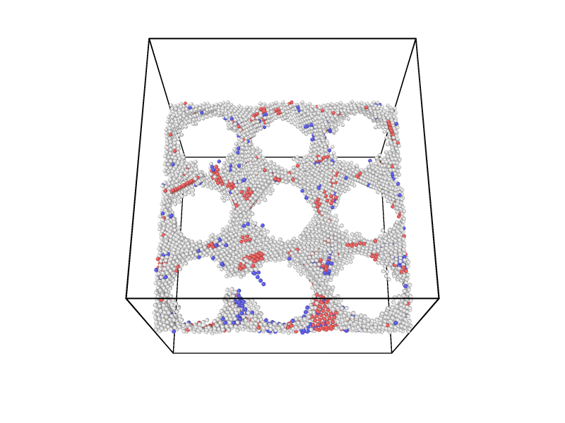
First, we add a SliceModifier to the pipeline, which cuts out a thin slab of material, to obtain
an unobstructed view of the grain boundary network.
The call to add_to_scene() is important: only pipelines that are part of the three-dimensional scene
appear in rendered images. A Viewport defines the virtual camera, and zoom_all()
adjusts the camera position such that the entire dataset is visible. The resulting image shows the grain boundary atoms,
colored by structure type.
See Rendering & visualization to learn how to control the visual appearance of the data, the camera, and the rendering engine.
The complete script
Here is the complete Python script, which you can save to a file and run with a Python interpreter, e.g. python quickstart.py:
# Step 1: Load the simulation data
from ovito.io import import_file

pipeline = import_file("NanocrystallinePd.dump.gz")

# Step 2: Inspect the loaded data
data = pipeline.compute()
print("Number of atoms:", data.particles.count)
print("Particle properties:", list(data.particles.keys()))

# Step 3: Add an analysis modifier to the pipeline
from ovito.modifiers import CommonNeighborAnalysisModifier

pipeline.modifiers.append(CommonNeighborAnalysisModifier())

# Step 4: Evaluate the pipeline and access the results
import numpy

data = pipeline.compute()
fcc_count = data.attributes["CommonNeighborAnalysis.counts.FCC"]
print(f"Fraction of fcc atoms: {fcc_count / data.particles.count:.1%}")

structure_types = data.particles["Structure Type"]
print("Atoms per structure type:", numpy.bincount(structure_types))

# Step 5: Extend the pipeline
from ovito.modifiers import SelectTypeModifier, DeleteSelectedModifier

pipeline.modifiers.append(SelectTypeModifier(
    property="Structure Type",
    types={CommonNeighborAnalysisModifier.Type.FCC}))
pipeline.modifiers.append(DeleteSelectedModifier())

# Step 6: Export the results to files
from ovito.io import export_file

export_file(pipeline, "grain_boundary_atoms.dump", "lammps/dump",
            columns=["Particle Identifier", "Structure Type", "Position.X", "Position.Y", "Position.Z"])
export_file(pipeline, "structure_counts.txt", "txt/table", key="structures")

# Step 7: Render an image
from ovito.modifiers import SliceModifier
from ovito.vis import Viewport

pipeline.modifiers.append(SliceModifier(normal=(0, 0, 1), slab_width=15))
pipeline.add_to_scene()
viewport = Viewport(type=Viewport.Type.Perspective, camera_dir=(0, 0.4, -1))
viewport.zoom_all()
viewport.render_image(filename="grain_boundaries.png", size=(800, 600))
Where to go from here
Data pipelines explains how pipelines work, including how to process simulation trajectories consisting of many frames.
Data model and Manipulating data show how to access and modify the data in a
DataCollection.User-defined modifiers shows how to implement your own analysis algorithms in Python and insert them into a pipeline.
Code examples contains more complete example scripts.